Spheres, de Sitter Continuation, and Outlook

The previous two pages used Rindler coordinates to show that a familiar vacuum can look thermal when viewed through a horizon. The final step of the course is to recognize that this was not an isolated trick. The same analytic structure appears whenever a Lorentzian problem can be obtained by continuing a smooth Euclidean geometry.

The cleanest compact example is the sphere. For a real, free, minimally coupled scalar with $m^2>0$, the Green function on $S^2$ is the covariance of a positive Euclidean Gaussian and can be found by expanding in spherical harmonics. Continuing one angular coordinate gives two-dimensional de Sitter space, and the regular Euclidean covariance selects the time-oriented Wightman function of the Euclidean, or Bunch–Davies, state. The massless constant mode requires separate treatment below. The thermal behavior of a static observer follows from the same mechanism as the Unruh temperature: a smooth Euclidean origin fixes an imaginary-time period.

This page has two jobs. First, it closes the geometric thread: polar coordinates, Rindler wedges, spheres, and de Sitter horizons are all expressions of the same analytic-continuation principle. Second, it records the final blackboard hints of the course: gauge/string ideas, order–disorder variables, fermionic-string questions, and turbulence are not separate curiosities but natural continuations of the methods developed here.

Required background. Unruh temperature and thermal periodicity supplies KMS analyticity, Euclidean regularity, and observer-dependent Hamiltonians.

Helpful background. Rindler coordinates and Green functions gives the flat-space continuation that de Sitter generalizes, while in–out, in–in, and Schwinger–Keldysh functionals motivates the nonequilibrium outlook.

Worldline sources and closed real-time contours

Geometry conventions. For formulas involving de Sitter space we keep the mostly-minus Lorentzian signature used throughout the course. Thus the global $dS_2$ metric is written as

$$ds^2=R^2\left(dT^2-\cosh^2T\,d\alpha^2\right), \qquad \alpha\sim\alpha+2\pi.$$

The corresponding Euclidean sphere has positive metric

$$ds_E^2=R^2\left(d\theta^2+\cos^2\theta\,d\alpha^2\right).$$

The continuation $\theta=iT$ gives $ds_E^2=-ds^2$, as expected under Wick rotation. It is useful to define the de Sitter invariant

$$Z(x,x')=-{X\cdot X'\over R^2},$$

where the ambient metric is $dX_0^2-dX_1^2-dX_2^2$ and the hyperboloid obeys $X\cdot X=-R^2$. With this definition, $Z=1$ at coincident points.

What the Euclidean continuation selects. The Euclidean sphere does three jobs at once. It gives a regulator-friendly compact spectral problem, fixes a regular short-distance singularity, and selects a Lorentzian state by analyticity. It does not mean that Lorentzian global time is periodic or that every observer sees the same Hamiltonian. Thermal behavior appears after choosing a static patch and restricting to the observables accessible inside its horizon.

Status of the course-end outlook. The sphere and static-patch calculations below are derivations. The later gauge/string, order–disorder, and turbulence sections expand the manuscript’s closing prompts into signposts; they do not claim to derive those subjects from the preceding de Sitter calculation.

First consider a worldline source in flat Minkowski coordinates. A point particle with coupling $q$ moving on a trajectory $x^\mu(s)$ defines the distributional current

$$J^\mu(x) =q\int_C ds\,\dot x^\mu(s)\, \delta^{(d)}\!\big(x-x(s)\big).$$

Its coupling to a gauge field may be written either as a spacetime integral or as a line integral:

$$S_{\rm int} =\int d^dx\,J^\mu A_\mu =q\int_C A_\mu\,dx^\mu.$$

For a closed trajectory, $\partial_\mu J^\mu=0$ and the corresponding amplitude contains the Wilson factor

$$W_q(C)=\exp\!\left(iq\oint_C A_\mu\,dx^\mu\right).$$

An open worldline instead has endpoint sources in $\partial_\mu J^\mu$; it becomes gauge invariant only after its endpoints are attached to appropriately charged operators. This distinction is why closed loops are natural observables in a gauge theory. Here the delta function is normalized with the displayed flat measure. On a curved spacetime, the vector current instead uses the invariant delta $\delta_g$, normalized by $\int d^dx\,\sqrt{\lvert g\rvert}\,\delta_g(x,y)f(x)=f(y)$; the spacetime coupling uses the same measure and conservation is $\nabla_\mu J^\mu=0$ for a closed curve.

An amplitude uses one history, but a probability or expectation value multiplies an amplitude by its complex conjugate. With an initial density matrix $\rho_0$, the source-dependent object is

$$Z[J_+,J_-] =\operatorname{Tr}\!\left( U[J_+]\rho_0U^\dagger[J_-] \right).$$

The $+$ and $-$ sources live on forward and backward time branches. When their particle trajectories join, they form a closed contour—the real-time origin of the Wilson-loop picture and of the Schwinger–Keldysh formalism. After Wick rotation, a large rectangular loop with spatial width $R$ and Euclidean duration $T$ behaves as

$$\langle W(R,T)\rangle\sim e^{-T V(R)},$$

which extracts the static potential. The gauge/string outlook below asks when $V(R)$ remains linear at large $R$.

Dissipative dynamics makes the need for a closed real-time contour especially clear. A term such as $\gamma\dot x$ in $m\ddot x+\gamma\dot x=F$ changes sign under time reversal, and forcing or an initial state selects an arrow of time even when the underlying microscopic theory is reversible. Equilibrium KMS relations strongly constrain the two contour branches; a generic driven state does not obey those constraints.

From the sphere to de Sitter space

Start with the unit two-sphere embedded in Euclidean $\mathbb R^3$:

$$n_0^2+n_1^2+n_2^2=1.$$

A convenient parametrization is

$$n_0=\sin\theta, \qquad n_1=\cos\theta\cos\alpha, \qquad n_2=\cos\theta\sin\alpha,$$

with metric

$$ds_E^2=d\theta^2+\cos^2\theta\,d\alpha^2.$$

Restoring the radius $R$ multiplies the metric by $R^2$. Now continue

$$\theta=iT.$$

Since $\sin(iT)=i\sinh T$ and $\cos(iT)=\cosh T$, the continued embedding is equivalent to

$$X_0=R\sinh T, \qquad X_1=R\cosh T\cos\alpha, \qquad X_2=R\cosh T\sin\alpha.$$

These coordinates satisfy

$$X_0^2-X_1^2-X_2^2=-R^2.$$

This is the one-sheeted de Sitter hyperboloid. Pulling back the ambient metric $dX_0^2-dX_1^2-dX_2^2$ gives

$$\boxed{ ds^2=R^2\left(dT^2-\cosh^2T\,d\alpha^2\right). }$$

Thus the compact Euclidean sphere has become a Lorentzian spacetime whose spatial slices are circles that shrink to a minimum at $T=0$ and grow like $e^{|T|}$ at early and late global time.

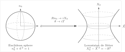
The sphere $n_0^2+\vec n^{\,2}=1$ becomes the de Sitter hyperboloid $X_0^2-\vec X^{\,2}=-R^2$ after continuing one embedding coordinate, or equivalently one angular coordinate. The compact Euclidean problem supplies a preferred analytic continuation of Green functions.

The invariant that replaces the Euclidean dot product is

$$Z(x,x')=-{X\cdot X'\over R^2}.$$

In global coordinates,

$$\boxed{ Z=\cosh T\cosh T'\cos(\alpha-\alpha')-\sinh T\sinh T'. }$$

At coincidence $Z=1$. In a convex normal neighborhood, let $\sigma(x,x')$ be half the signed squared geodesic interval. Then

$$Z=1+{\sigma\over R^2} +O\!\left({\sigma^2\over R^4}\right).$$

Thus $1-Z$ is negative for nearby timelike points and positive for nearby spacelike points. At equal angle, $Z=\cosh(T-T')$; at $T=T'=0$, $Z=\cos(\alpha-\alpha')$. These two checks fix the signs directly. The Wightman boundary value must additionally retain the time orientation of the pair, as in Spradlin, Strominger, and Volovich 2001, §3.1, pp.12–14 (PDF).

The lesson is the same as for Rindler space, but now global rather than local. In Rindler, Euclidean polar coordinates

$$ds_E^2=d\rho^2+\rho^2d\theta^2$$

become Lorentzian boost coordinates after $\theta=i\eta$. In de Sitter, an angular coordinate of the sphere becomes global time. Smooth Euclidean geometry is doing the work.

Green functions from the sphere

Let $\phi$ be a real, free, minimally coupled scalar on $S^2_R$, with $m^2>0$. Its Euclidean action is $\frac12\int_{S^2_R}dV\,[(\nabla\phi)^2+m^2\phi^2]$, so the two-point function is the covariance given by the inverse of the positive elliptic operator

$$-\nabla_{S^2_R}^2+m^2.$$

It solves

$$\left(-\nabla_{S^2_R}^2+m^2\right)G_E(\Omega,\Omega') =\delta_{S^2_R}(\Omega,\Omega').$$

Because the sphere is rotationally invariant, $G_E$ depends only on

$$z=n\cdot n'=\cos\gamma,$$

where $\gamma$ is the geodesic angle between the two points on the unit sphere. The spherical harmonics satisfy

$$-\nabla_{S^2_{\rm unit}}^2Y_{\ell m}=\ell(\ell+1)Y_{\ell m},$$

and the addition theorem gives

$$\sum_{m=-\ell}^{\ell}Y_{\ell m}(\Omega)Y_{\ell m}^*(\Omega')={2\ell+1\over4\pi}P_\ell(z).$$

Writing

$$M^2=m^2R^2,$$

we obtain

$$\boxed{ G_E(z)=\sum_{\ell=0}^{\infty}{2\ell+1\over4\pi} {P_\ell(z)\over \ell(\ell+1)+M^2}. }$$

Every harmonic eigenvalue is positive for $M^2=m^2R^2>0$. For a real test function with harmonic coefficients $f_{\ell m}$ on the unit sphere, the covariance quadratic form is $\sum_{\ell m}\lvert f_{\ell m}\rvert^2/[\ell(\ell+1)+M^2]\geq0$. Invertibility alone would not imply this positivity. The Euclidean and Bunch–Davies free-field discussion explains the state-selection conditions; the Legendre formula here is specifically two-dimensional.

The figure separates the positive Euclidean covariance from the analytic continuation and its time-oriented Lorentzian boundary value.

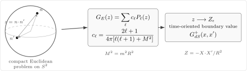
For the real minimally coupled scalar with $M^2=m^2R^2>0$, the harmonic inverse is a positive Euclidean covariance. Its analytic continuation, with the time-oriented boundary value $Z_\epsilon$, gives the Euclidean/BD Wightman function. The arrows show the construction schematically; they do not assert that the original Legendre series converges at every Lorentzian argument.

Symbolically, the Lorentzian de Sitter two-point function is obtained by continuing

$$z\longrightarrow Z_\epsilon.$$

More explicitly, the Euclidean, or Bunch–Davies, Wightman function is schematically

$$G^+_{dS}(x,x')=\lim_{\epsilon\to0^+}G_E\!\big(Z(x,x')-i\epsilon\,s(x,x')\big),$$

where $s(x,x')=\operatorname{sgn}(T-T')$ for timelike-separated pairs in the global time already defined: it is positive when $x$ is to the future of $x'$. A constant replacement $Z\mapsto Z-i0$ is only shorthand: the sign must retain the time orientation of the two points. One first continues the analytic Green function and then takes its distributional boundary value; substituting arbitrary Lorentzian $Z$ directly into a possibly nonconvergent Legendre series is not the prescription. Euclidean regularity and the oriented limit select the state Spradlin, Strominger, and Volovich 2001, §3.1, pp.12–14 (PDF).

A small but important exception occurs for a massless minimally coupled scalar. When $M^2=0$, the $\ell=0$ term is not invertible:

$${1\over \ell(\ell+1)+M^2}\bigg|_{\ell=0,M=0}\to\infty.$$

This is the compact-space version of an infrared zero mode. One must either remove the constant mode, add a small mass and take limits carefully, or study derivative operators whose correlators are insensitive to the constant shift. For the undifferentiated massless minimally coupled field, there is no ordinary de Sitter-invariant Fock vacuum with a finite field two-point function obtained by simply inverting the Laplacian. This caveat is not cosmetic; many de Sitter infrared puzzles begin with precisely this zero mode.

There are three pieces of physics packed into this simple prescription.

First, the state is de Sitter invariant: its boundary value depends on $Z$ together with the pair’s time orientation. Second, its short-distance singularity is the same as the flat-space Hadamard singularity, because a small patch of de Sitter space is locally Minkowskian. Third, the positive massive Euclidean construction selects a distinguished vacuum. In an expanding spacetime, “positive frequency” is often ambiguous; analyticity inherited from the compact Euclidean sphere is a much better guide.

A useful check is the large-mass or short-distance limit. If the separation is much smaller than $R$, then the sphere looks locally like a plane and

$$1-z\simeq {\gamma^2\over2}.$$

The Green function reduces locally to the two-dimensional Euclidean massive propagator. After continuation, this becomes the local Minkowski Wightman singularity with the usual $i0$ prescription. Curvature changes the global analytic structure, not the leading ultraviolet singularity.

Static-patch thermality

Global de Sitter time is not the time measured by a static observer. To see the thermal statement, use static-patch coordinates. In $dS_2$ they may be written as

$$X_0=\sqrt{R^2-r^2}\,\sinh {\tau\over R},$$ $$X_1=\sqrt{R^2-r^2}\,\cosh {\tau\over R}, \qquad X_2=r.$$

The induced metric is

$$\boxed{ ds^2=\left(1-{r^2\over R^2}\right)d\tau^2 -\left(1-{r^2\over R^2}\right)^{-1}dr^2. }$$

The coordinate patch covers $|r|<R$. The surfaces $r=\pm R$ are horizons for the static observer. They are the de Sitter analogue of Rindler horizons.

Now Wick rotate

$$\tau=-i\tau_E.$$

The Euclidean metric is

$$ds_E^2=\left(1-{r^2\over R^2}\right)d\tau_E^2 +\left(1-{r^2\over R^2}\right)^{-1}dr^2.$$

Near the horizon, put $r=R-y$ with $y\ll R$. Then

$$1-{r^2\over R^2}\simeq {2y\over R}.$$

Define

$$\rho=\sqrt{2Ry}.$$

A short calculation gives

$$ds_E^2\simeq d\rho^2+\rho^2\left({d\tau_E\over R}\right)^2.$$

This is the Euclidean plane in polar coordinates. Smoothness at $\rho=0$ therefore requires

$${\tau_E\over R}\sim {\tau_E\over R}+2\pi,$$

or

$$\boxed{ \tau_E\sim \tau_E+2\pi R. }$$

Thermal field theory identifies the Euclidean time period with inverse temperature. Hence a static observer at $r=0$ sees

$$\boxed{ T_{dS}={1\over2\pi R}. }$$

This is the Gibbons–Hawking temperature of de Sitter space.

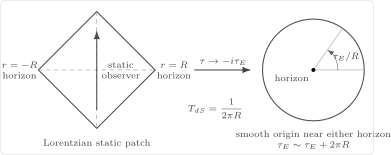
The Lorentzian static patch has horizons at $r=\pm R$. After Wick rotation, each horizon is locally a smooth Euclidean origin. Avoiding a conical singularity fixes $\tau_E\sim\tau_E+2\pi R$. The displayed $T_{dS}=1/(2\pi R)$ refers to the Killing generator of $\tau$, normalized to proper time at $r=0$; the local temperature at other radii includes the lapse below.

At nonzero $r$, the local proper time is redshifted:

$$dt_{\rm proper}=\sqrt{1-{r^2\over R^2}}\,d\tau.$$

Therefore the locally measured temperature is

$$\boxed{ T_{\rm local}(r)={1\over2\pi R\sqrt{1-r^2/R^2}}. }$$

It diverges near the horizon in the same way that the local Unruh temperature diverges for a Rindler observer held closer and closer to the horizon.

Occupation numbers and what is thermal

The thermal statement should be phrased with respect to a specified time generator. In the static patch, $H_{\rm st}$ generates $\tau$ translations. Write $\omega>0$ for the corresponding Killing-energy gap. A static detector in the Euclidean de Sitter state, in its stationary weak-coupling and long-time response regime, satisfies detailed balance,

$${\Gamma_\uparrow\over\Gamma_\downarrow}=e^{-2\pi R\omega}.$$

If the detector’s fixed proper-time gap is $\Omega$, its phase is $e^{-i\Omega t_{\rm proper}}=e^{-iN(r)\Omega\tau}$, where $N(r)=\sqrt{1-r^2/R^2}>0$. Consequently

$$\omega=N(r)\Omega, \qquad {\Gamma_\uparrow\over\Gamma_\downarrow} =e^{-2\pi R N(r)\Omega} =e^{-\Omega/T_{\rm local}(r)}.$$

This combines the Euclidean-state detector calculation Spradlin, Strominger, and Volovich 2001, §3.2, pp.15–17 (PDF) with the proper-time redshift derived above. The Tolman–KMS discussion develops the same distinction for general stationary equilibrium.

For bosonic modes, this corresponds to

$$\boxed{ n_B(\omega)={1\over e^{2\pi R\omega}-1}. }$$

For fermionic modes,

$$\boxed{ n_F(\omega)={1\over e^{2\pi R\omega}+1}. }$$

For comparison, a homogeneous equilibrium state in flat Minkowski spacetime can be written using a constant future-directed unit four-velocity $u^\mu$, rest-frame inverse temperature $\beta_0$, and chemical potential $\mu_0$. With well-defined conserved translation charges $P^\mu$ and internal charge $Q$, and a thermal trace or its appropriate equilibrium limit, the expression is

$$\rho={1\over Z} \exp\left[-\beta_0\left(u_\mu P^\mu-\mu_0Q\right)\right].$$

For $u^\mu=\gamma(1,\mathbf v)$, a one-particle state contributes $u\cdot p=\gamma(E_{\mathbf p}-\mathbf v\cdot\mathbf p)$, so

$$n_{B/F}(\mathbf p) = {1\over \exp\left\{ \beta_0\left[ \gamma(E_{\mathbf p}-\mathbf v\cdot\mathbf p)-\mu_0q \right]\right\}\mp1}.$$

The denominator has $-1$ for bosons and $+1$ for fermions, within the domain where the equilibrium ensemble exists. Writing $\beta(E-\mathbf v\cdot\mathbf p-\mu q)$ gives the same exponent when $\beta=\gamma\beta_0$ and $\mu=\mu_0/\gamma$. This is a flat-space boost relation. On a static curved background, equilibrium instead refers to a specified timelike Killing flow and its normalization; its position-dependent norm produces the Tolman redshift. A constant Minkowski thermal vector cannot replace that construction. In particular, global de Sitter $\partial_T$ is not Killing, since the spatial metric depends on $T$.

This is why the distinction between global and static de Sitter time matters. The Euclidean state is de Sitter invariant, but a particular observer’s thermal bath is defined relative to the observer’s causal patch and Killing time. Thermal behavior is not merely a property of the state; it is a property of the pair consisting of a state and an algebra of accessible observables.

Gauge/string hints

The course has repeatedly used the idea that long-distance physics may be better described by extended objects than by the microscopic fields in the Lagrangian. Wilson loops diagnose confinement by asking whether the gauge field creates an effective string worldsheet. For an external probe that cannot be screened by dynamical matter, an asymptotic area law has the form

$$\langle W(R,T)\rangle\sim e^{-\sigma RT},$$

so the static potential is

$$V(R)=\sigma R.$$

The coefficient $\sigma$ is a string tension. A relativistic string with tension $T_s$ has Regge-like behavior

$$J\simeq \alpha' M^2+a, \qquad \alpha'={1\over2\pi T_s}$$

for open strings, up to intercept and quantum corrections. Closed strings have a related but different slope; in the simplest flat-space normalization the leading closed-string slope is half the open-string slope. The point is not the exact intercept. The point is dimensional: a string tension turns angular momentum into a quantity proportional to energy squared.

If dynamical matter can screen the probe, the flux tube can break and the asymptotic Wilson loop need not retain an area law. The monopole-confinement lesson gives an explicit example: odd center charge remains confined, while an even-charge string breaks on the massive $W$ bosons.

This is the seed of the gauge/string viewpoint. In gauge theory, flux tubes and Wilson surfaces suggest stringy degrees of freedom. In string theory, a two-dimensional worldsheet field theory produces spacetime particles. A Lorentzian warped background with a spatial radial coordinate $\varphi$ and real positive warp factor $a(\varphi)$ has the form

$$ds^2=-d\varphi^2+a^2(\varphi)\,\eta_{\mu\nu}dx^\mu dx^\nu.$$

The radial minus sign leaves exactly one timelike direction; it is not an extra ambient embedding time. For $a(\varphi)=e^{\varphi/L}$, the change $z=L e^{-\varphi/L}$ gives

$$ds^2={L^2\over z^2} \left(\eta_{\mu\nu}dx^\mu dx^\nu-dz^2\right), \qquad z>0.$$

This is the Poincaré AdS metric in the site’s convention. Its radial null rays obey $dt=\pm dz$ at fixed boundary spatial coordinates. The transformation $(x^\mu,z)\mapsto(c x^\mu,c z)$, $c>0$, is an isometry, illustrating the relation between radial position and boundary scale Aharony et al. 2000, §2.2.1, pp.42–43, Eqs.(2.27)–(2.28) (PDF). The AdS geometry discussion develops the one-time metric and its conformal boundary.

In a suitable holographic theory, $\varphi$ can act as an energy-scale coordinate and the warp factor changes tensions measured in the $x^\mu$ directions. An arbitrary warp factor alone does not establish a Wilsonian flow or a dual field theory; that identification also requires a consistent bulk dynamics and a boundary dictionary.

These comments are deliberately only a doorway. The calculational foundations laid earlier in the course — beta functions, operator products, sigma models, instantons, large-$N$ methods, and Wilson loops — are precisely the tools that make the gauge/string correspondence more than an analogy.

Order–disorder variables and the fermionic-string question

Another thread running through the course is that the best variables are often nonlocal in the original variables. In two-dimensional statistical systems, order and disorder operators are the simplest example. In the Ising model, the spin field $\sigma$ and the disorder field $\mu$ have nontrivial monodromy with each other. With a branch prescription and the appropriate angular factors, their operator product contains the chiral fermion fields schematically as

$$\sigma\times\mu\sim \psi+\bar\psi.$$

This says that fermionic operators can arise from the mutual branch structure of bosonic order and disorder variables. Bosonization, duality, and the Schwinger model pages were all variations on this theme: locality depends on which algebra of operators one chooses as fundamental.

In higher dimensions, a disorder operator is defined by a prescribed singularity or monodromy on a surface that links its support. Its support may be local, line-like, or surface-like depending on the dimension and the symmetry: a monopole operator in three spacetime dimensions can be local, while Wilson and ’t Hooft operators are lines. There is no rule that disorder operators in three dimensions must be extended.

The manuscript’s phrase “fermionic string” is therefore best read as a research question, not a universal construction. An extended excitation can carry fermionic worldsheet degrees of freedom or require spin/framing data, but that claim must be established in a specific model by its operator algebra and exchange properties. The Ising order–disorder OPE motivates the question; it does not by itself prove that a given gauge-theory flux tube is fermionic.

This also explains why the course spent so much time on Wilson loops, theta terms, monopoles, and instantons. Nonperturbative operators are not optional decorations. They are often the variables in which the phase of the theory is simplest.

Turbulence and nonequilibrium field theory

A natural final outlook is turbulence, which may look like a sharp turn away from QFT. It is not. Turbulence is a field theory of many degrees of freedom, scale transfer, composite operators, and anomalous scaling. The difference is that the system is not in equilibrium.

For an incompressible velocity field,

$$\partial_i v_i=0,$$

the Navier–Stokes equation is

$$\partial_t v_i+v_j\partial_jv_i=-\partial_i p+\nu\nabla^2v_i+f_i.$$

Here $f_i$ is an external stirring force and $\nu$ is the viscosity. For Gaussian stirring, one may specify a transverse covariance

$$\langle f_i(t,\mathbf x)f_j(t',\mathbf x')\rangle =\delta(t-t')D_{ij}(\mathbf x-\mathbf x'), \qquad \partial_iD_{ij}=0.$$

A stochastic formulation introduces a response field $\tilde v_i$ and turns correlation functions into a path integral of Martin–Siggia–Rose/Janssen–De Dominicis type. Suppressing the incompressibility projectors and the response-field contour, the action is schematically

$$\begin{aligned} S_{\rm MSR} ={}& \int dt\,d^dx\,\tilde v_i \left( \partial_t v_i+v_j\partial_jv_i +\partial_i p-\nu\nabla^2v_i \right) \\ &-{1\over2} \int dt\,d^dx\,d^dx'\, \tilde v_i(t,\mathbf x) D_{ij}(\mathbf x-\mathbf x') \tilde v_j(t,\mathbf x'). \end{aligned}$$

The pressure or an explicit transverse projector enforces $\partial_iv_i=0$. This looks like a field theory, but it is not a Euclidean equilibrium theory. In a driven–dissipative steady state there is no automatic KMS relation or reflection positivity, and detailed time reversal is generally broken. The Schwinger–Keldysh and in–in ideas from the previous pages are therefore the right conceptual relatives.

The RG question is also familiar. In the usual three-dimensional direct-energy-cascade regime, large-scale forcing and a much shorter viscous dissipation scale leave an intermediate inertial range with approximate scaling. The direction is not universal: two-dimensional incompressible flow also conserves enstrophy in the inviscid limit and can transfer energy toward larger scales while enstrophy moves toward smaller scales Kraichnan 1967, §1, p.1417 (PDF). The dimension, forcing, dissipation, and range of scales are part of the physical question. Composite operators and their anomalous dimensions become central, linking scale dependence to real-time dynamics.

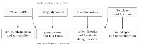
The late-course outlook is not a list of unrelated topics. RG, OPE, gauge dynamics, topology, horizons, and low-dimensional dualities become entry points to critical phenomena, gauge/string ideas, order–disorder constructions and fermionic-string questions, curved-space QFT, and nonequilibrium field theory.

Course-end checklist

A useful way to leave the course is to name the recurring moves:

Move	Earlier example	Later avatar
integrate out short distances	Wilsonian RG and OPE	effective strings and hydrodynamic actions
sum topological sectors	instantons and monopoles	theta dependence, confinement, vacuum decay
change variables nonlocally	bosonization and disorder operators	dual photons, Wilson loops, string variables
choose the right real-time contour	in–in formalism	pair creation, transport, turbulence
continue from a smooth Euclidean problem	Rindler polar plane	de Sitter and horizon thermality

These are not separate tricks. They are different ways of keeping observables, symmetries, and causal structure under control while changing the variables appropriate to the scale, state, or observer.

Summary

The analytic continuation from $S^2$ to $dS_2$ is the compact cousin of the Rindler continuation from a Euclidean plane to a Lorentzian wedge. For the real free scalar with $m^2>0$, the sphere’s discrete spectral inverse is a positive covariance. Its analytic continuation to the time-oriented boundary value $Z_\epsilon$ selects the Euclidean, or Bunch–Davies, Lorentzian correlator. Invertibility alone is insufficient for a physical covariance, and the massless constant mode remains a separate problem.

The thermal character of de Sitter space follows from Euclidean smoothness. In the static patch, the horizon becomes the origin of a Euclidean disk, and regularity fixes the imaginary-time period $2\pi R$. A static observer therefore sees the de Sitter temperature $T=1/(2\pi R)$, with the usual redshift for observers away from $r=0$.

The broader lesson is that QFT is a language for changing descriptions. Short-distance effects are organized by local operators. Some strongly coupled gauge systems admit descriptions in terms of flux tubes or monopole gases. Two-dimensional bosonic and fermionic theories can encode the same observables. Restricting a vacuum across a horizon can produce a thermal KMS state for the accessible algebra. Nonequilibrium systems require real-time contours rather than Euclidean partition functions. The course ends not by closing these topics, but by showing that the same tools keep reappearing.

Common pitfalls

Making Lorentzian global time periodic. The Euclidean sphere does not imply periodic global de Sitter time. The thermal period is in imaginary static time and is tied to a horizon and an observer.

Calling de Sitter thermality observer independent. The Bunch–Davies state is de Sitter invariant, but “thermal” is a patch statement. A static observer describes the restricted state thermally with respect to the static Hamiltonian.

Inverting the massless scalar zero mode. For a massless minimally coupled scalar on a compact sphere, the $\ell=0$ mode makes the field Green function singular. Remove the constant mode, regulate the mass, or use shift-invariant observables; do not silently apply the massive formula.

Treating $Z-i0$ as a constant complex shift. A Wightman boundary value needs a sign fixed by time orientation. The shorthand $Z-i0$ is insufficient when the ordering of the two points is not already specified.

Promoting the outlook to established consequences. The Regge and warped-metric formulas are controlled within string models, not exact spectra of arbitrary confining gauge theories. The “fermionic string” phrase is a model-dependent question, not a theorem.

Confusing nonequilibrium dynamics with Wick rotation. Real-time expectation values require closed time paths or response-field formalisms. A driven–dissipative state has no automatic KMS relation.

Exercises

Exercise 1: Spectral inverse on the sphere

Let $G_E(z)$ on a unit $S^2$ be expanded as

$$G_E(z)=\sum_{\ell=0}^{\infty}a_\ell P_\ell(z).$$

Using

$$\delta_{S^2}(\Omega,\Omega')=\sum_{\ell=0}^{\infty}{2\ell+1\over4\pi}P_\ell(n\cdot n')$$

and

$$-\nabla_{S^2}^2P_\ell(n\cdot n')=\ell(\ell+1)P_\ell(n\cdot n'),$$

find $a_\ell$ for the Green function of $-\nabla^2+M^2$ with $M^2>0$.

Solution

We require

$$(-\nabla^2+M^2)G_E(\Omega,\Omega')=\delta_{S^2}(\Omega,\Omega').$$

Substituting the Legendre expansion gives

$$\sum_{\ell=0}^{\infty}a_\ell\left[\ell(\ell+1)+M^2\right]P_\ell(z) = \sum_{\ell=0}^{\infty}{2\ell+1\over4\pi}P_\ell(z).$$

Matching coefficients of $P_\ell(z)$ yields

$$a_\ell={2\ell+1\over4\pi}\,{1\over\ell(\ell+1)+M^2}.$$

Therefore

$$G_E(z)=\sum_{\ell=0}^{\infty}{2\ell+1\over4\pi} {P_\ell(z)\over\ell(\ell+1)+M^2}.$$

For $M^2>0$, every harmonic covariance eigenvalue $1/[\ell(\ell+1)+M^2]$ is positive. This condition has content beyond invertibility: the formal parameter $M^2=-1/2$ gives no zero eigenvalue, but the normalized constant harmonic would have variance $-2$, which cannot be a real Gaussian covariance. If $M^2=0$, the $\ell=0$ coefficient diverges; the constant zero mode cannot be inverted without imposing an additional condition or removing the zero mode.

Exercise 2: Continuing the metric

Start from

$$ds_E^2=R^2(d\theta^2+\cos^2\theta\,d\alpha^2).$$

Set $\theta=iT$ and show that the corresponding mostly-minus Lorentzian metric is

$$ds^2=R^2(dT^2-\cosh^2T\,d\alpha^2).$$

Then compute the embedding invariant $Z=-X\cdot X'/R^2$ in global coordinates.

Solution

The continuation gives

$$d\theta^2=-dT^2, \qquad \cos\theta=\cosh T.$$

Thus

$$ds_E^2=R^2(-dT^2+\cosh^2T\,d\alpha^2).$$

Under Wick rotation, the Euclidean metric is the negative of the mostly-minus Lorentzian metric, so

$$ds^2=-ds_E^2=R^2(dT^2-\cosh^2T\,d\alpha^2).$$

The embedding coordinates are

$$X_0=R\sinh T, \qquad X_1=R\cosh T\cos\alpha, \qquad X_2=R\cosh T\sin\alpha.$$

With ambient product

$$X\cdot X'=X_0X_0'-X_1X_1'-X_2X_2',$$

we get

$${X\cdot X'\over R^2}=\sinh T\sinh T'-\cosh T\cosh T'\cos(\alpha-\alpha').$$

Therefore

$$Z=-{X\cdot X'\over R^2} =\cosh T\cosh T'\cos(\alpha-\alpha')-\sinh T\sinh T'.$$

At coincidence, $Z=1$.

Exercise 3: De Sitter temperature from smoothness

For the static-patch metric

$$ds^2=f(r)d\tau^2-f(r)^{-1}dr^2, \qquad f(r)=1-{r^2\over R^2},$$

derive the Euclidean period of $\tau_E$ required for smoothness at $r=R$.

Solution

After Wick rotation $\tau=-i\tau_E$, the Euclidean metric is

$$ds_E^2=f(r)d\tau_E^2+f(r)^{-1}dr^2.$$

Near $r=R$, write $r=R-y$ with $y\ll R$. Then

$$f(r)=1-{(R-y)^2\over R^2}\simeq {2y\over R}.$$

Define

$$\rho=\sqrt{2Ry}.$$

Then

$$dy={\rho\over R}d\rho,$$

and

$$f^{-1}dr^2=f^{-1}dy^2\simeq {R\over2y}{\rho^2\over R^2}d\rho^2=d\rho^2.$$

Also,

$$f d\tau_E^2\simeq {2y\over R}d\tau_E^2={\rho^2\over R^2}d\tau_E^2.$$

Thus

$$ds_E^2\simeq d\rho^2+\rho^2\left({d\tau_E\over R}\right)^2.$$

This is smooth polar form only if

$${\tau_E\over R}\sim {\tau_E\over R}+2\pi.$$

Therefore

$$\tau_E\sim\tau_E+2\pi R, \qquad T={1\over2\pi R}.$$

Exercise 4: Redshifted local temperature

A static observer at fixed $r$ has proper time

$$dt_{\rm proper}=\sqrt{1-r^2/R^2}\,d\tau.$$

If the thermal period in $\tau_E$ is $2\pi R$, find the local temperature measured by this observer.

Solution

The Euclidean period in the coordinate time is

$$\beta_\tau=2\pi R.$$

The proper Euclidean time period is redshifted:

$$\beta_{\rm proper}=\sqrt{1-r^2/R^2}\,\beta_\tau =2\pi R\sqrt{1-r^2/R^2}.$$

The locally measured temperature is the inverse proper period:

$$T_{\rm local}(r)={1\over\beta_{\rm proper}} ={1\over2\pi R\sqrt{1-r^2/R^2}}.$$

It equals $1/(2\pi R)$ at $r=0$ and diverges as $r\to R$, reflecting the infinite acceleration required to remain static at the horizon.

Exercise 5: From detailed balance to occupation numbers

Suppose a bosonic oscillator mode of frequency $\omega$ is coupled to a thermal bath. Detailed balance says

$${\Gamma_\uparrow\over\Gamma_\downarrow}=e^{-\beta\omega}.$$

If the upward rate is proportional to $n_B(\omega)$ and the downward rate is proportional to $1+n_B(\omega)$, derive the Bose–Einstein occupation number.

Solution

The ratio of rates is

$${\Gamma_\uparrow\over\Gamma_\downarrow} ={n_B(\omega)\over1+n_B(\omega)}.$$

Detailed balance therefore gives

$${n_B\over1+n_B}=e^{-\beta\omega}.$$

Solving,

$$n_B=e^{-\beta\omega}(1+n_B),$$

so

$$n_B(1-e^{-\beta\omega})=e^{-\beta\omega}.$$

Hence

$$n_B={1\over e^{\beta\omega}-1}.$$

For the static patch of de Sitter space, $\beta=2\pi R$ when $\omega$ is a Killing-energy gap. For a static detector with proper gap $\Omega$, the same exponent is $\beta\omega=2\pi R N(r)\Omega$; equivalently use $\beta_{\rm proper}=2\pi R N(r)$ with $\Omega$.

Exercise 6: Zero mode on the sphere

For a massless scalar on a compact unit sphere, explain why the equation

$$-\nabla^2 G(\Omega,\Omega')=\delta_{S^2}(\Omega,\Omega')$$

has no solution unless the zero mode is removed. Show that the modified equation

$$-\nabla^2 G_0(\Omega,\Omega')= \delta_{S^2}(\Omega,\Omega')-{1\over4\pi}$$

is compatible with integration over the sphere.

Solution

Integrate the naive equation over $\Omega$:

$$\int_{S^2}d\Omega\,[-\nabla^2G(\Omega,\Omega')] =\int_{S^2}d\Omega\,\delta_{S^2}(\Omega,\Omega')=1.$$

But the integral of a Laplacian over a compact manifold without boundary vanishes:

$$\int_{S^2}d\Omega\,\nabla^2G=0.$$

Thus the left side is zero while the right side is one, a contradiction. The problem is the constant zero mode of $-\nabla^2$.

For the modified equation,

$$\int_{S^2}d\Omega\,\left[\delta_{S^2}(\Omega,\Omega')-{1\over4\pi}\right] =1-{1\over4\pi}\int_{S^2}d\Omega=1-1=0.$$

Now the source is orthogonal to the constant mode, so the equation can be solved after fixing the additive constant of $G_0$.

References

• O. Aharony, S. S. Gubser, J. Maldacena, H. Ooguri, and Y. Oz, “Large N Field Theories, String Theory and Gravity,” Physics Reports 323 (2000), 183–386, doi:10.1016/S0370-1573(99)00083-6, Open PDF, arXiv:hep-th/9905111v3.
• B. Allen, “Vacuum States in de Sitter Space,” Physical Review D 32 (1985), 3136–3149, doi:10.1103/PhysRevD.32.3136.
• T. S. Bunch and P. C. W. Davies, “Quantum Field Theory in de Sitter Space: Renormalization by Point-Splitting,” Proceedings of the Royal Society of London A 360 (1978), 117–134, doi:10.1098/rspa.1978.0060.
• D. Forster, D. R. Nelson, and M. J. Stephen, “Large-Distance and Long-Time Properties of a Randomly Stirred Fluid,” Physical Review A 16 (1977), 732–749, doi:10.1103/PhysRevA.16.732.
• G. W. Gibbons and S. W. Hawking, “Cosmological Event Horizons, Thermodynamics, and Particle Creation,” Physical Review D 15 (1977), 2738–2751, doi:10.1103/PhysRevD.15.2738.
• R. H. Kraichnan, “Inertial Ranges in Two-Dimensional Turbulence,” The Physics of Fluids 10 (1967), 1417–1423, doi:10.1063/1.1762301, Open PDF.
• M. Spradlin, A. Strominger, and A. Volovich, “Les Houches Lectures on de Sitter Space,” lecture notes, arXiv:hep-th/0110007v1 (2001), arXiv record, Open PDF, cited preprint pagination.

Further reading

• N. D. Birrell and P. C. W. Davies, Quantum Fields in Curved Space, Cambridge Monographs on Mathematical Physics, Cambridge University Press, Cambridge, 1982.
• U. Frisch, Turbulence: The Legacy of A. N. Kolmogorov, Cambridge University Press, Cambridge, 1995.
• C. Itzykson and J.-M. Drouffe, Statistical Field Theory, vol. 1, Cambridge Monographs on Mathematical Physics, Cambridge University Press, Cambridge, 1989.
• J. Polchinski, String Theory, vol. 1, Cambridge Monographs on Mathematical Physics, Cambridge University Press, Cambridge, 1998.
• A. M. Polyakov, Gauge Fields and Strings, Contemporary Concepts in Physics, vol. 3, Harwood Academic Publishers, Chur, 1987.