Anti-de Sitter Geometry and the Conformal Boundary

Anti-de Sitter space is the maximally symmetric Lorentzian geometry whose universal cover has a timelike conformal boundary. That one sentence carries most of the geometric input to AdS/CFT: the radius fixes the curvature scale, the covering space removes closed timelike curves, the boundary supplies only a conformal class, and the timelike character of that boundary means that initial data alone do not in general determine bulk evolution. None of these facts, by itself, selects a boundary condition, a quantum state, or a dual conformal field theory.

Required background. Smooth manifolds, tangent spaces, and tensors supplies induced metrics and curvature tensors. Helpful background. Conformal geometry and compactification supplies the boundary action of the conformal group, while timelike AdS boundaries develops the general evolution problem.

We will first derive the global metric from an embedding, then bring infinity to a finite conformal boundary, and finally verify that the ambient isometries act conformally there. A convention round trip checks that these results do not depend on copying one source’s sign choices.

The AdS hyperboloid and its universal cover

Let the ambient space $\mathbb R^{2,d}$ have coordinates $X^A=(X_{-1},X_0,X_1,\ldots,X_d)$ and line element

$$\mathrm ds_{\mathrm{amb}}^2 =\mathrm dX_{-1}^2+\mathrm dX_0^2 -\sum_{i=1}^{d}\mathrm dX_i^2.$$

AdS$_{d+1}$ of radius $L$ is the connected hyperboloid

$$X_{-1}^2+X_0^2-\sum_{i=1}^{d}X_i^2=L^2$$

with the induced metric. The two plus signs belong to the ambient construction; the hyperboloid itself has one timelike direction. Parametrize it by

$$\begin{aligned} X_{-1}&=L\cosh\rho\cos\tau, &X_0&=L\cosh\rho\sin\tau,\\ X_i&=L\sinh\rho\,n_i, &\sum_{i=1}^{d}n_i^2&=1. \end{aligned}$$

The unit vector $n_i$ obeys $n_i\mathrm dn_i=0$ and $\mathrm dn_i\mathrm dn_i=\mathrm d\Omega_{d-1}^2$, the metric of the unit $(d-1)$-sphere. Differentiating the two coordinate blocks gives

$$\begin{aligned} \mathrm dX_{-1}^2+\mathrm dX_0^2 &=L^2\left(\sinh^2\rho\,\mathrm d\rho^2 +\cosh^2\rho\,\mathrm d\tau^2\right),\\ \sum_i\mathrm dX_i^2 &=L^2\left(\cosh^2\rho\,\mathrm d\rho^2 +\sinh^2\rho\,\mathrm d\Omega_{d-1}^2\right). \end{aligned}$$

Subtracting the spatial block and using $\cosh^2\rho-\sinh^2\rho=1$ produces the global metric

$$\mathrm ds^2=L^2\left( \cosh^2\rho\,\mathrm d\tau^2 -\mathrm d\rho^2 -\sinh^2\rho\,\mathrm d\Omega_{d-1}^2 \right).$$

If $\gamma_{ab}$ is the unit-sphere metric, then the block determinant gives

$$\sqrt{\lvert g\rvert} =L^{d+1}\cosh\rho\,\sinh^{d-1}\rho\, \sqrt{\det\gamma}.$$

The embedding is periodic under $\tau\mapsto\tau+2\pi$. On the hyperboloid, a curve at fixed $\rho$ and angles is therefore a closed timelike curve. In holography, “global AdS” almost always means the universal cover obtained by unwrapping $\tau$ to the real line. Its topology is $\mathbb R\times\mathbb R^d$, while a constant-$\tau$ slice is hyperbolic space $H^d$. This global choice is additional to the local curvature tensor Aharony et al. 2000, §2.2.1, eqs. (2.20)–(2.23).

Bringing infinity to a finite coordinate boundary

Introduce $\chi$ by

$$\tan\chi=\sinh\rho, \qquad 0\leq\chi<\frac{\pi}{2}.$$

Then $\cosh\rho=\sec\chi$ and

$$\mathrm ds^2=\frac{L^2}{\cos^2\chi} \left( \mathrm d\tau^2-\mathrm d\chi^2 -\sin^2\chi\,\mathrm d\Omega_{d-1}^2 \right).$$

The defining function $\Omega=\cos\chi/L$ vanishes at $\chi=\pi/2$ with $\mathrm d\Omega\neq0$. The rescaled metric $\bar g=\Omega^2g$ is regular there and induces the dimensionless boundary representative

$$\mathrm d\bar s_{\partial}^2 =\mathrm d\tau^2-\mathrm d\Omega_{d-1}^2.$$

The boundary of the universal cover has topology $\mathbb R_\tau\times S^{d-1}$. Its normal is spacelike in $\bar g$, so the boundary is timelike. For $d=1$, $S^0$ consists of two points, and this notation describes the two timelike boundary components of AdS$_2$. The boundary is not a wall at finite physical distance: along a radial spacelike curve beginning at any fixed $\chi_0<\pi/2$,

$$\ell=L\int_{\chi_0}^{\pi/2}\frac{\mathrm d\chi}{\cos\chi}=\infty.$$

Conformal rescaling preserves null trajectories but not affine parameters. A radial null curve obeys

$$\mathrm d\tau=\pm\mathrm d\chi,$$

so a ray emitted from the center reaches the conformal boundary after the finite global-time interval $\Delta\tau=\pi/2$ Aharony et al. 2000, §2.2.1, eqs. (2.24)–(2.25). To display both radial directions along one chosen diameter, define a signed coordinate $\sigma=\chi$ on one ray and $\sigma=-\chi$ on its antipodal ray, so $\lvert\sigma\rvert=\chi$. The radial section below separates the geometric first arrival from a return that assumes reflecting boundary data.

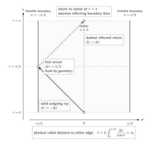
In this schematic $1+1$-dimensional radial section, the conformal boundaries lie at signed radial coordinate $\sigma=\pm\pi/2$, although their physical proper distance is infinite. The solid leg is fixed by the null equation and reaches the boundary at $\Delta\tau=\pi/2$; the dashed return to the center at $\tau=\pi$ is conditional on reflecting boundary data. For $d>1$, the two edges represent antipodal points of the boundary sphere along one diameter; for $d=1$, they are the two boundary components. The diagram is not to scale.

Because information can enter from the timelike boundary, a spacelike slice is not a Cauchy surface by itself. For a linear field, the mathematical rule that completes evolution is a domain for the spatial wave operator. Admissibility may select a unique positive self-adjoint extension in some sectors; when several positive extensions exist, the remaining choice is boundary behavior. Reflection, absorption into a declared exterior, or another rule belongs to the completed dynamical problem, not to the conformal diagram alone Ishibashi and Wald 2004, §§1 and 3.3.

Boundary conformal class, scale, and time evolution

A defining function is not unique. Replacing $\Omega$ by $e^\omega\Omega$, with $e^\omega$ positive and regular at the boundary, changes the induced representative by

$$g_{(0)}\longmapsto e^{2\omega}g_{(0)}.$$

The intrinsic boundary datum is therefore the conformal class $[g_{(0)}]$, not one preferred metric. A convenient dimensionful representative is

$$\mathrm ds_{(0)}^2 =L^2\left(\mathrm d\tau^2-\mathrm d\Omega_{d-1}^2\right),$$

whose cylinder radius is $L$ and whose physical time is $t_{\mathrm{cyl}}=L\tau$.

If a boundary CFT admits radial quantization and the state–operator map, a primary $\mathcal O$ of dimension $\Delta$ creates a cylinder state $\lvert\mathcal O\rangle$ obeying

$$(H_{\mathrm{cyl}}-E_{\mathrm{vac}}\mathbf 1) \lvert\mathcal O\rangle =\frac{\Delta}{L}\lvert\mathcal O\rangle, \qquad (E_{\mathrm{cyl}}-E_{\mathrm{vac}})L=\Delta$$

In Euclidean radial quantization, the flat-space dilatation generator $\mathcal D$ generates logarithmic radial time; after the flat-space-to-cylinder identification, its eigenvalues become cylinder energies Aharony et al. 2000, §§2.1.1 and 3.4.2, especially eq. (3.77). This is a kinematic statement about a boundary theory with the state–operator map. Pure AdS geometry supplies the cylinder time, but it does not supply $\mathcal D$, $E_{\mathrm{vac}}$, or a dual Hilbert space. The later states and radial quantization page develops the dictionary.

From ambient isometries to boundary conformal maps

The boundary action can be checked without choosing a Poincaré chart. Divide the embedding coordinates by their common large-$\rho$ scale:

$$P^A(\tau,n) =\lim_{\rho\to\infty}\frac{X^A}{L\cosh\rho} =(\cos\tau,\sin\tau,n_i), \qquad P^AP_A=0.$$

A boundary point is an oriented null ray, $P^A\sim\lambda P^A$ for $\lambda>0$; the universal cover additionally unwraps $\tau$. On the displayed section of the null cone,

$$\mathrm dP^2=\mathrm d\tau^2-\mathrm d\Omega_{d-1}^2.$$

Let $M\in SO_0(2,d)$. The vector $MP$ is again null, but restoring the chosen section generally requires a position-dependent positive rescaling,

$$\widehat P(x')=\lambda(x)MP(x).$$

Since $P^2=P\mathbin{\cdot}\mathrm dP=0$ and $M$ preserves the ambient inner product,

$$\mathrm d\widehat P^2=\lambda(x)^2\mathrm dP^2.$$

Thus every connected ambient isometry induces a boundary transformation that preserves the metric up to a Weyl factor. The rotation in the $(X_{-1},X_0)$ plane gives the simplest example: it sends $\tau\mapsto\tau+\alpha$ and becomes cylinder time translation. At Lie-algebra level,

$$\mathfrak{isom}(\widetilde{\mathrm{AdS}}_{d+1}) \cong\mathfrak{so}(2,d) \cong\mathfrak{conf}_{\mathrm{global}} \!\left(\overline{\mathbb R^{1,d-1}}\right).$$

The last action is global on conformally compactified Minkowski space; a special conformal transformation need not preserve one chosen Minkowski patch. This projective-null-cone construction is the direct geometric verification of the symmetry match Witten 1998, §1.

Group-level qualifications remain. The universal cover, disconnected components, centers, and discrete quotients affect the allowed representations. In $d=2$, the classical local algebra is Witt $\oplus$ Witt and its quantum central extension is Virasoro $\oplus$ Virasoro, whereas $\mathfrak{so}(2,2)$ is the finite-dimensional global subalgebra. In $d=1$, local metric conformality alone is too weak to select a finite algebra; the oriented-null-ray and global AdS structure selects $\mathfrak{so}(2,1)$. Geometry therefore supplies a compatibility condition, not a CFT spectrum, global form, state space, or exact duality. The Gubser–Klebanov–Polyakov–Witten prescription adds dynamical field and source data to this geometric stage Witten 1998, §§2–3.

Curvature signs and the convention round trip

QFT.org uses signature $(+,-,\ldots,-)$ and

$$[\nabla_M,\nabla_N]V^P=R^P{}_{QMN}V^Q, \qquad R_{MNPQ}=g_{MR}R^R{}_{NPQ}.$$

The ambient normal $N^A=X^A/L$ has $N^AN_A=+1$, and its second fundamental form is $K_{MN}=\pm g_{MN}/L$. With the displayed Riemann convention, the flat-ambient-space Gauss equation is

$$R_{MNPQ}=K_{MP}K_{NQ}-K_{MQ}K_{NP}.$$

The normal-orientation sign cancels, leaving

$$R_{MNPQ}=\frac{1}{L^2} \left(g_{MP}g_{NQ}-g_{MQ}g_{NP}\right),$$

and hence

$$R_{MN}=\frac d{L^2}g_{MN}, \qquad R=\frac{d(d+1)}{L^2}.$$

For the vacuum equation $G_{MN}+\Lambda g_{MN}=0$, these tensors require

$$\Lambda=\frac{d(d-1)}{2L^2}.$$

These plus signs are the internally consistent mostly-minus form of AdS. To translate to a mostly-plus metric while retaining the displayed commutator convention, set $g'=-g$. Then

$$\Gamma'=\Gamma, \quad R'^P{}_{QMN}=R^P{}_{QMN}, \quad R'_{MN}=R_{MN}, \quad G'_{MN}=G_{MN},$$

whereas

$$R'=-R, \qquad R'_{MNPQ}=-R_{MNPQ}, \qquad \Box_{g'}=-\Box_g.$$

Consequently,

$$\begin{aligned} R'_{MN}&=-\frac d{L^2}g'_{MN},\\ R'_{MNPQ}&=-\frac1{L^2} \left(g'_{MP}g'_{NQ}-g'_{MQ}g'_{NP}\right),\\ \Lambda'&=-\Lambda=-\frac{d(d-1)}{2L^2}. \end{aligned}$$

The site equation $(\Box_g+m^2)\phi=0$ becomes $(\Box_{g'}-m^2)\phi=0$ after multiplying the equation by $-1$. Meanwhile $g(v,v)=0$ if and only if $g'(v,v)=0$, so the null curves, radial equation, timelike character of the boundary, and conformal diagram are unchanged. The curvature-squared invariant also survives:

$$R_{MNPQ}R^{MNPQ}=\frac{2d(d+1)}{L^4}.$$

This is the adversarial check: if one flips only the Ricci tensor, $\Lambda$, or the wave operator without the correlated changes above, the strongest surviving statement is merely that a coordinate line element has been written—not that it realizes the declared AdS convention package.

What AdS geometry determines—and what it leaves open

Local geometry fixes the radius, curvature tensors, volume element, null cones, and isometry algebra. These are exact identities for pure AdS$_{d+1}$ with $L>0$; $L$ sets a scale rather than an approximation parameter.

A global spacetime choice fixes whether the time circle is unwrapped, the resulting boundary topology, and any quotient or spin-structure data. Those choices are invisible to local curvature invariants.

Boundary dynamics and state data fix the domain of each field equation, any boundary behavior not already selected by admissibility, and the bulk state. The self-adjoint-extension statement is a conditional classification for specified linear fields on fixed AdS, not a theorem about arbitrary interacting quantum gravity.

A candidate duality must supply the boundary theory, operator and normalization map, global sectors, state dictionary, approximation regime, and evidence. The embedding, compactification, and $\mathfrak{so}(2,d)$ action establish a necessary geometric stage; they do not establish a holographic equivalence. The mathematical identities above have no residual numerical uncertainty, while the existence and completeness of any proposed duality are separate, theory-dependent claims.

Common pitfalls

Treating the compactified boundary as a finite-distance wall. It lies at finite coordinate position in $\bar g$ but at infinite proper radial distance in the physical metric $g$. Compactification preserves causal relations, not physical lengths.

Letting the diagram choose the reflection rule. Geometry fixes the first arrival at the boundary. A reflected return requires the field equation and admissible boundary data.

Equating a symmetry match with a duality. The same $SO(2,d)$ structure is necessary for an AdS/CFT pairing, but it neither constructs a CFT nor proves that bulk and boundary observables agree.

Translating one sign in isolation. Metric signature, Riemann convention, Einstein equation, wave operator, and curvature coupling form a package. Use the unchanged null diagram and curvature-squared invariant as round-trip checks.

Exercises

Pull back the ambient metric

Starting from the embedding coordinates, derive the global AdS metric and its volume density. Explain where $n_i\mathrm dn_i=0$ is used.

Solution: induced metric and measure

Differentiating $n_in_i=1$ gives $n_i\mathrm dn_i=0$. This removes the mixed $\mathrm d\rho\,\mathrm dn_i$ term from $\sum_i\mathrm dX_i^2$. The time-plane block and spatial block are

$$\begin{aligned} \mathrm dX_{-1}^2+\mathrm dX_0^2 &=L^2\left(\sinh^2\rho\,\mathrm d\rho^2 +\cosh^2\rho\,\mathrm d\tau^2\right),\\ \sum_i\mathrm dX_i^2 &=L^2\left(\cosh^2\rho\,\mathrm d\rho^2 +\sinh^2\rho\,\mathrm d\Omega_{d-1}^2\right). \end{aligned}$$

Their signed difference gives the displayed metric. Its diagonal blocks contribute $L^2\cosh^2\rho$, $-L^2$, and $-L^2\sinh^2\rho\,\gamma_{ab}$, so taking the absolute determinant yields

$$\sqrt{\lvert g\rvert} =L^{d+1}\cosh\rho\,\sinh^{d-1}\rho\sqrt{\det\gamma}.$$

Compactification and radial light travel

Use $\tan\chi=\sinh\rho$ to obtain the compactified metric. Show that its boundary is timelike and that a radial light ray emitted from the center at $\tau=0$ first reaches it at $\tau=\pi/2$. What extra assumption is needed for the ray to return to the center at $\tau=\pi$?

Solution: boundary and null travel

From $\cosh\rho=\sec\chi$ and $\mathrm d\rho=\sec\chi\,\mathrm d\chi$, substitution gives

$$\mathrm ds^2=\frac{L^2}{\cos^2\chi} \left(\mathrm d\tau^2-\mathrm d\chi^2 -\sin^2\chi\,\mathrm d\Omega_{d-1}^2\right).$$

In the regular metric $\bar g$, the normal to $\chi=\pi/2$ has negative norm in the mostly-minus convention and is spacelike; its boundary hypersurface is therefore timelike. A radial null curve has $\mathrm d\tau=\pm\mathrm d\chi$. Integrating the outgoing branch from $0$ to $\pi/2$ gives $\Delta\tau=\pi/2$. A second leg back to the center requires reflecting boundary data; the conformal diagram alone does not supply it.

Verify the boundary conformal action

Show that $P^A=(\cos\tau,\sin\tau,n_i)$ is null and that its induced metric is the cylinder representative. Then prove that $\widehat P=\lambda(x)MP$, with $M\in SO_0(2,d)$, changes that metric only by the Weyl factor $\lambda^2$.

Solution: projective null cone

The ambient norm is

$$P^2=\cos^2\tau+\sin^2\tau-n_in_i=0.$$

Because $n_i\mathrm dn_i=0$ and $\mathrm dn_i\mathrm dn_i=\mathrm d\Omega_{d-1}^2$,

$$\mathrm dP^2=\mathrm d\tau^2-\mathrm d\Omega_{d-1}^2.$$

Now differentiate $\widehat P=\lambda MP$. Terms proportional to $(MP)^2$ vanish because $P^2=0$, and cross terms vanish because $P\mathbin{\cdot}\mathrm dP=\tfrac12\mathrm d(P^2)=0$. Since $M$ preserves the ambient product, the remaining term is

$$\mathrm d\widehat P^2=\lambda^2\mathrm dP^2.$$

Thus the action on null rays is conformal. A rotation in the two ambient timelike coordinates has $\lambda=1$ and becomes the exact cylinder isometry $\tau\mapsto\tau+\alpha$.

Reverse the metric signature

Set $g'=-g$ while holding fixed the displayed definition of $R^P{}_{QMN}$. Determine the changes in $\Gamma$, $R^P{}_{QMN}$, $R_{MNPQ}$, $R_{MN}$, $R$, $G_{MN}$, $\Lambda$, and $\Box$. Explain why the boundary causal diagram is unchanged.

Solution: convention round trip

The inverse metric also changes sign, so the two signs in the Levi-Civita connection cancel: $\Gamma'=\Gamma$. Hence $R'^P{}_{QMN}=R^P{}_{QMN}$ and its Ricci contraction is unchanged. Lowering the first index introduces one sign, while tracing the Ricci tensor with the inverse metric introduces one sign:

$$R'_{MNPQ}=-R_{MNPQ}, \qquad R'_{MN}=R_{MN}, \qquad R'=-R.$$

The two signs in $Rg_{MN}$ cancel, so $G'_{MN}=G_{MN}$. The same written vacuum equation then needs $\Lambda'=-\Lambda$ because $g'_{MN}=-g_{MN}$. Finally $\Box_{g'}=-\Box_g$. Since multiplication by $-1$ does not change which tangent vectors are null, it leaves every null trajectory and the causal diagram unchanged.

Global, Poincaré, and AdS-Rindler Patches next asks which part of this geometry a coordinate chart and its time generator cover. Timelike-Boundary Causality and Boundary-Value Problems supplies the data needed for evolution. Theorem-level reconstruction and boundary-net questions belong to Mathematical QFT.

The chapter overview contains the structure diagram and validity and failure diagram. They are embedded there once so that their shared chapter-level context is not repeated on every article.

For the chapter-wide comparison of assumptions, counterevidence, falsifiers, and claim ceilings, see the claim-domain table.

References

• Aharony, Ofer, Steven S. Gubser, Juan Maldacena, Hirosi Ooguri, and Yaron Oz. “Large N Field Theories, String Theory and Gravity.” Physics Reports 323 (2000): 183–386. arXiv. DOI.
• Ishibashi, Akihiro, and Robert M. Wald. “Dynamics in Non-Globally-Hyperbolic Static Spacetimes III: Anti-de Sitter Spacetime.” Classical and Quantum Gravity 21 (2004): 2981–3014. arXiv. DOI.
• Witten, Edward. “Anti-de Sitter Space and Holography.” Advances in Theoretical and Mathematical Physics 2 (1998): 253–291. arXiv. DOI.