Traversable Wormholes, Couplings, and Energy Conditions

A two-sided AdS black hole can acquire a temporary traversable window when a deliberately timed interaction between its two boundary theories induces negative renormalized null energy on the horizon. The resulting gravitational response advances an early probe far enough to emerge from the opposite exterior. Entanglement alone does not do this: the sign of the interaction, its retarded support, the probe’s wave packet, and the probe’s own positive-energy backreaction all matter.

This page derives that chain twice. First, the Gao–Jafferis–Wall (GJW) horizon calculation turns a complete horizon average into a boundary-anchored, causally meaningful opening shift after a Kruskal normalization is fixed. Then a nearly-AdS$_2$ benchmark gives an explicit leading time advance and a finite-energy signaling window. The conclusion is deliberately narrow: a controlled semiclassical channel exists for specified states, operators, timing, and couplings—not an autonomous macroscopic shortcut or a violation of causality in the coupled boundary system.

Required background. Lorentzian Einstein–Rosen Bridges and Two-Boundary States fixes the uncoupled state. Averaged Null Energy Condition supplies the null-energy diagnostic. Shockwaves, OTOCs, and Scrambling supplies the near-horizon scattering regime.

Helpful background. Quantum Energy Inequalities in Curved Spacetime and Quantum Interest and Negative-Energy Compensation constrain negative energy. Quantum Communication and Entanglement Distribution separates a channel from shared entanglement.

The interaction changes the causal problem

Begin with identical large-$N$ theories in the thermofield-double state. Let $t_L$ and $t_R$ both increase toward the physical future, as on the preceding causal and boundary-time map. A brief scalar coupling at equal physical times is

$$\delta H(\tau) =-\int d^{d-1}\mathbf x\, h(\tau,\mathbf x)\, O_L(\tau,\mathbf x)O_R(\tau,\mathbf x),$$

where $d$ is the boundary spacetime dimension. GJW instead write $O_R(t)O_L(-t)$ because their single Schwarzschild Killing coordinate increases toward the physical future on the right and toward the physical past on the left. The two expressions agree after setting $t_R=t$ and $t_L=-t$ in that Killing-coordinate notation. This conversion prevents an easy but consequential sign and timing error.

If both scalar operators have dimension $\Delta$, then

$$[h]=\text{mass}^{d-2\Delta}.$$

The original ultraviolet-controlled example uses a relevant deformation, $2\Delta<d$, a smooth or finitely supported switching function, and a bulk scalar in the alternative-quantization window. In BTZ, $d=2$ and the result below applies for $0<\Delta<1$. These assumptions are part of the result, not disposable decoration.

For a sharply localized pulse and $K$ independent light fields, it is useful to write

$$U_g=\exp(ig\mathcal V), \qquad \mathcal V=\frac{1}{K}\sum_{j=1}^{K}O_L^j(0)O_R^j(0), \qquad \widetilde g=\frac{g}{K}\ll1.$$

This follows from $U_g=\exp[-i\int d\tau\,\delta H(\tau)]$. The total $g$ may be large in the nearly-AdS$_2$ benchmark while the coupling per species $\widetilde g$ remains small.

The Hamiltonian sign fixes the Kubo sign. For any later operator $B$,

$$\begin{aligned} \delta\langle B(t)\rangle &=i\int_{-\infty}^{t}dt'\, \langle[\delta H(t'),B(t)]\rangle_0 \\ &=-i\int_{-\infty}^{t}dt'\,d^{d-1}\mathbf x\, h(t',\mathbf x) \langle[O_L(t',\mathbf x)O_R(t',\mathbf x),B(t)]\rangle_0 . \end{aligned}$$

Reversing $h$ reverses the leading response. A formula with the same Hamiltonian but the opposite Kubo sign would describe a different convention and cannot be mixed into the later shift test.

From the boundary pulse to negative horizon energy

At large $N$, the double-trace insertion changes the bulk scalar two-point function before it changes the classical metric. In the homogeneous BTZ calculation, the first-order correction has the retarded structure

$$\begin{aligned} \delta G_{RR}(x,x') =2\sin(\pi\Delta)\int dt_1\,d\phi_1\, h(t_1,\phi_1)\, K_{LR}(x';t_1,\phi_1)K_{\mathrm{ret}}(x;t_1,\phi_1) +(x\leftrightarrow x'). \end{aligned}$$

The cross-boundary kernel $K_{LR}$ contains the TFD correlation; the retarded kernel makes the causal ordering explicit. Point splitting then gives

$$\delta\langle T_{UU}(U)\rangle_{\mathrm{ren}} =\lim_{U'\to U}\partial_U\partial_{U'}\delta G(U,U'),$$

on the horizon $V=0$. For the relevant BTZ scalar, positive $h$ in the Hamiltonian convention above, and $0<\Delta<1$, GJW find

$$\mathcal E_U \equiv\int_{-\infty}^{+\infty}dU\, \delta\langle T_{UU}(U)\rangle_{\mathrm{ren}}<0.$$

The local stress can develop a positive late-time tail; traversability is governed by the complete horizon integral, not by the sign at one point. The calculation and its sign are given in Gao, Jafferis, and Wall 2017, §§ 2–3 and eq. (3.18).

Here $U$ is affine on the undeformed horizon. Under an orientation-preserving affine rescaling $U'=aU+b$, $\mathcal E_{U'}=\mathcal E_U/a$; its sign is invariant, but its magnitude is not. Every comparison among the opening shift, the signal shock, and the packet width must therefore use one fixed Kruskal normalization.

This negative horizon average does not contradict an achronal-ANEC theorem. Once the two boundaries are directly coupled, points on the relevant complete generator can be joined through the boundary interaction, so the generator is chronal and the achronal theorem’s hypotheses no longer hold. The correct statement is “negative complete horizon-averaged null energy in the specified coupled system,” not “a counterexample to every ANEC result” Gao, Jafferis, and Wall 2017, § 1, especially pp. 3–5.

From horizon energy to a geometric opening

Let $D=d+1\geq3$ be the bulk spacetime dimension, $r_h$ the horizon radius, and $L$ the AdS radius. Write $q_{UU}=\delta g_{UU}$ so it is not confused with the boundary coupling $h$. In the spherically symmetric linearized problem, define

$$C_h\equiv\frac{D-3}{r_h^2}+\frac{D-1}{L^2}>0.$$

Integrating the $UU$ Einstein equation over the complete $V=0$ generator removes the total derivatives and gives

$$8\pi G_N\mathcal E_U =\frac{D-2}{4}C_h \int_{-\infty}^{+\infty}dU\,q_{UU}(U).$$

In the GJW-oriented Kruskal chart, where $g_{UV}^{(0)}(0)<0$, the perturbed horizon ray obeys

$$V(U)=-\frac{1}{2g_{UV}^{(0)}(0)} \int_{-\infty}^{U}dU'\,q_{UU}(U').$$

Rather than attaching physical meaning to the convention-dependent sign of $V$, define the positive opening magnitude

$$\begin{aligned} \alpha_{\mathrm{open}} &\equiv -V(+\infty) \\ &=\frac{16\pi G_N}{(D-2)C_h\lvert g_{UV}^{(0)}(0)\rvert} \bigl(-\mathcal E_U\bigr)>0 . \end{aligned}$$

Thus the sign chain is explicit: the chosen boundary pulse gives $\mathcal E_U<0$, the integrated metric perturbation moves the marginal ray to the escaping side, and $\alpha_{\mathrm{open}}>0$. The prefactor is specific to the symmetric mode and the declared coordinate normalization. A transversely localized perturbation instead requires the appropriate shock Green function. These relations reproduce Gao, Jafferis, and Wall 2017, eqs. (1.3)–(1.5).

The figure separates this geometric opening from the boundary interaction that creates it. Inspect the dotted uncoupled trajectory, the solid transmitted trajectory, and the three failure exits; the line joining the two coupling events is explicitly a boundary interaction and not a curve through the bulk. The drawing chooses left-to-right transmission for readability; exchanging the identical sides gives the right-to-left benchmark used below.

On a narrow screen, swipe or use the Left and Right arrow keys to pan across the figure. Home and End move to its edges. A full-size link is also available.

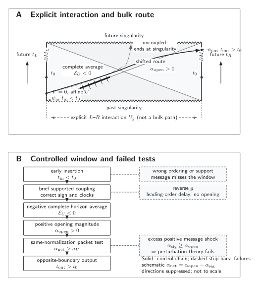
Schematic pulsed double-trace protocol in one declared Kruskal normalization. A brief explicit left–right interaction makes the complete renormalized horizon average negative and produces an opening shift. An early probe reaches the opposite boundary only when the causal ordering is correct and its positive-energy backreaction leaves a net shift larger than the packet width. Reversing the sign or missing the retarded support closes the derived window; excessive backreaction either closes it or invalidates the perturbative calculation. The coupling is itself a communication resource; this is neither an autonomous wormhole nor a quantitative macroscopic geometry. Not to scale. Accessible figure data (JSON)

The same control logic in linear form is:

Case	Boundary operation	Horizon average	Shift test	Causal outcome	Validity statement
Uncoupled baseline	No left–right interaction	Deformation-induced $\delta\mathcal E_U=0$	$\alpha_{\mathrm{open}}=0$	An infalling signal ends at the singularity	Exact no-signaling between dynamically decoupled factors
Correct sign and ordering	Brief $U_g$ with $t_{\mathrm{in}}<t_0<t_{\mathrm{out}}$	$\mathcal E_U<0$ in the stated model	$\alpha_{\mathrm{net}}>\sigma_V$	A supported wave packet can emerge	Semiclassical, retarded, and perturbative regime only
Reversed sign	$U_{-g}$	Leading sign reverses	Delay rather than opening	No traversable route	First-order sign control
Wrong ordering	Pulse and message have no required retarded support	The pulse may still change the state	The message does not sample the opening	No through-bulk signal for that protocol	Operator ordering and support are essential
Excessive signal energy	Correct pulse plus a large positive-energy message shock	Negative source average need not disappear	$\alpha_{\mathrm{net}}\leq\sigma_V$ or perturbation theory fails	Channel closes or the leading calculation becomes inconclusive	Must use the backreacted correlator or nonlinear geometry

Here $\sigma_V$ is the packet width in the same Kruskal coordinate. The message travels along the other null direction and carries $T_{VV}$ in this chart; its nonlinear or eikonal cross-shock backreaction degrades the correlations that create the opening. It is useful to summarize that effect by a positive effective closing contribution $\alpha_{\mathrm{sig}}$ and write

$$\alpha_{\mathrm{net}} =\alpha_{\mathrm{open}}-\alpha_{\mathrm{sig}}.$$

This is schematic same-normalization bookkeeping, not a subtraction of two $T_{UU}$ horizon integrals. Transmission requires $\alpha_{\mathrm{net}}>\sigma_V$, not merely a locally negative stress tensor. When the eikonal or perturbative approximation fails, the formula no longer establishes either opening or closure.

A reproducible nearly-AdS₂ time advance

The nearly-AdS$_2$ calculation makes the leading shift and its timing concrete. Use the source normalization $\beta=2\pi$ and symmetric boundary insertions

$$t_R=-t, \qquad t_L=+t, \qquad t>0,$$

with the pulse $U_g$ at time zero. The message therefore enters from the right before the pulse and is read on the left after it. Near the horizon, the relative boost produces the eikonal phase

$$S_{\mathrm{eik}}= \exp\!\left(iG_Ne^t p_+q_-\right),$$

where a physical message has $p_+<0$. Let

$$\lambda\equiv G_Ne^t .$$

For $g\gg1$, $\lambda\ll1$, and $g\lambda$ fixed, the local-operator probe expression can be obtained by expanding the backreacted integrand. That expansion is controlled for a smeared physical packet only when the momenta carrying appreciable wave-function support also obey $|p_+|\lambda\ll1$. When the coupling operator and message operator have the same dimension $\Delta$, the source-normalized local correlator reduces to a translated vacuum correlator,

$$C_{\mathrm{probe}}(t) =\left\langle\phi_L e^{-ia^+P_+}\phi_R\right\rangle =\frac{1}{\left(2+a^+/2\right)^{2\Delta}},$$

with

$$a^+ =-\frac{\Delta g}{2^{2\Delta+1}}\,G_Ne^t =-\frac{\Delta g}{2^{2\Delta+1}}\,\lambda .$$

Positive $g$ gives $a^+<0$, a time advance in these coordinates. The idealized local correlator reaches the light cone at $a^+=-4$ and acquires the causal discontinuity associated with a nonzero left–right commutator beyond it. Smearing the message over boundary time replaces the local-operator singularity by a finite crossover, as a physical wave packet should. The derivation and general-time expression are in Maldacena, Stanford, and Yang 2017, §§ 2.2–2.3 and eqs. (2.16)–(2.21).

Numerical control fixture

Choose dimensionless parameters

$$\Delta=0.7, \qquad g=10^4, \qquad \lambda=G_Ne^t=4.0\times10^{-3}.$$

Also take $K\gg10^4$, so that the per-species coupling $\widetilde g=g/K\ll1$ even though the collective coupling is large.

Then

$$a^+ =-\frac{0.7\times10^4}{2^{2.4}} \left(4.0\times10^{-3}\right) \simeq-5.31<-4.$$

The arithmetic places the ideal local-operator formula beyond its source-normalized light-cone threshold while $\lambda\ll1$. It does not by itself specify a controlled packet: one must still choose smearing whose relevant momenta satisfy $|p_+|\lambda\ll1$ and then include its finite width and backreaction. If, illustratively, $G_N=10^{-6}$ in this normalization, then $t=\log(4000)\simeq8.29$, or $t_{\mathrm{phys}}\simeq(\beta/2\pi)8.29$ after restoring units. The benchmark is internally reproducible as a local-probe threshold check, but it is not a universal prediction: changing $\Delta$, the pulse profile, the packet smearing, or the Kruskal normalization changes the numerical threshold data.

Two controls are immediate. Replacing $g$ by $-g$ gives $a^+\simeq+5.31$, a delay. Moving the message insertion to the wrong side of the pulse removes the out-of-time-ordered scattering configuration that generated the exponentially enhanced response. Neither control permits the probe-level crossing.

The finite-energy signaling window

The probe formula cannot be extrapolated to an arbitrarily energetic or arbitrarily early message. For equal coupling and message dimensions, the leading eikonal correlator including the message’s backreaction is, in the same nearly-AdS$_2$ normalization,

$$\widetilde C =\frac{1}{\Gamma(2\Delta)} \int_{-\infty}^{0}\frac{dp_+}{-p_+}\, (2ip_+)^{2\Delta}e^{-4ip_+} \exp\!\left[ \frac{ig}{\left(2-p_+\lambda/2\right)^{2\Delta}} \right].$$

The power and exponential preceding the scattering phase are the exact local-operator wave-function overlap in this convention; for a smeared packet they are replaced by its actual overlap. Only the total $p_+$ enters the scattering phase for a multiparticle message. Because $p_+<0$, increasing $-p_+^{\mathrm{total}}$ suppresses the cross-boundary $OO$ correlator that created the opening. Independent propagation requires

$$\lambda\bigl(-p_+^{\mathrm{total}}\bigr)\lesssim1.$$

At the same time, a packet must be narrow enough to fit through the shift. Parametrically,

$$\Delta x^+\lesssim g\lambda, \qquad \Delta x^+\Delta p_+\gtrsim1, \qquad -p_+^{\mathrm{each}}\gtrsim\frac{1}{g\lambda}.$$

For $N_{\mathrm{send}}$ comparable packets, combining the lower bound on each momentum with the upper bound on total momentum gives

$$N_{\mathrm{send}} \sim\frac{-p_+^{\mathrm{total}}}{-p_+^{\mathrm{each}}} \lesssim g.$$

This is a parametric capacity bound, not a sharp one-qubit theorem; wave-packet shapes and order-one constants were suppressed. It shows why “send earlier” is not an unlimited strategy. Earlier insertion increases the boost and initially helps the opening, but it also magnifies the message shock until the source correlations are degraded and the probe picture closes. See Maldacena, Stanford, and Yang 2017, §§ 2.4–2.5 and eqs. (2.15)–(2.18), (2.22)–(2.27).

The controlled window therefore has four simultaneous requirements:

1. Retarded order: $t_{\mathrm{in}}<t_0<t_{\mathrm{out}}$, with the appropriate scattering ordering.
2. Opening sign: the chosen operator, state, and $g$ must give $\mathcal E_U<0$ and $\alpha_{\mathrm{open}}>0$.
3. Resolution: the net shift must exceed the packet width.
4. Backreaction control: the positive message shock and higher-order corrections must remain small enough that the retained approximation is self-consistent.

Failure of any one condition closes the derived channel. Outside the perturbative domain the honest conclusion is “not established by this calculation,” not “still open by continuity.”

Channel interpretation, causality, and energy bounds

The coherent double-trace unitary is a quantum entangling interaction between the two boundary systems. It is therefore already a communication resource. Maldacena, Stanford, and Yang also give a one-way implementation: measure the relevant operator on the sending side, communicate the ordinary classical outcome, and apply an outcome-dependent unitary on the receiving side. This reproduces the receiver’s reduced density matrix for the stated protocol, not the full global state Maldacena, Stanford, and Yang 2017, § 2.1.1.

That observation explains the teleportation language without turning correlation into signaling. The TFD supplies shared entanglement; the coupling or measurement-and-feed-forward supplies the channel; the bulk description says that, in the controlled code sector, the message follows a smooth interior trajectory. No information is transmitted before the boundary resource is available, and the construction does not create a faster route than the causal structure of the coupled system.

Energy-condition language needs the same care. Timelike quantum energy inequalities and quantum-interest results can constrain negative energy after a field theory, state class, sampling curve, and sampling function are fixed. There is no universal state-independent bound on every finite null segment in every dimension. QNEC is a local lower bound involving a null second variation of entropy; that lower bound can itself be negative, so QNEC is not the pointwise NEC Bousso et al. 2016, eq. (1.1). Deriving an ANEC statement from QNEC additionally requires control of the entropy-derivative endpoint terms, and the interacting-QFT proof has its own locality and deformation hypotheses Balakrishnan et al. 2019, §§ 2–4. Nor can a QEI for an ordinary local theory be transferred unchanged to a deliberately nonlocal interboundary coupling. The safe procedure is to calculate the renormalized stress in the actual model, evaluate the complete horizon average, and then test the applicable inequality hypotheses; Kontou 2024, §§ 2–4 reviews where QEI restrictions do and do not apply.

This protocol is also not generic quantum energy teleportation. QET can redistribute locally extractable energy using measurement, entanglement, and classical communication without a semiclassical wormhole dual. A gravitational traversability claim additionally requires the two-sided holographic state, a controlled bulk dictionary, negative horizon-averaged null energy, and the backreacted causal shift derived above.

Evidence and claim ceiling

Evidence checked 29 August 2026. The transient scalar construction is an analytic semiclassical result in BTZ and nearly-AdS$_2$ under the stated large-$N$, low-energy, operator, state, and switching assumptions. It is not universal over operators: conserved-current double-trace couplings give related but transport-dependent openings, for example through charge-diffusion data in black-brane models Ahn et al. 2024, §§ II–IV. A continuously coupled nearly-AdS$_2$/SYK ground state can instead support an eternal traversable solution, but that is a different Hamiltonian and phase problem, not the infinite-duration limit of this pulse calculation Maldacena and Qi 2018, §§ 2–4.

Statement	Status	Essential assumptions	Strongest licensed conclusion
The stated BTZ pulse gives $\mathcal E_U<0$	One-loop analytic model result	TFD, alternative-quantized scalar, $0<\Delta<1$, relevant smooth coupling, leading order	Negative complete horizon average for that model and sign
Negative $\mathcal E_U$ gives $\alpha_{\mathrm{open}}>0$	Linearized semiclassical gravity	Fixed affine/Kruskal normalization, symmetric mode or declared transverse kernel, controlled boundary terms	A marginal horizon ray is shifted to the escaping side
The unsmeared nearly-AdS$_2$ local probe reaches its light cone at $a^+=-4$	Source-normalized probe result	$g\gg1$, $G_Ne^t\ll1$, $gG_Ne^t$ fixed, declared operator dimensions	A smeared packet has a width-dependent finite crossover rather than a universal sharp threshold
Arbitrarily many or arbitrarily energetic messages cross	False extrapolation	Violates message-backreaction and wave-packet bounds	Parametrically $N_{\mathrm{send}}\lesssim g$ in the stated model
A small quantum processor realized a spacetime wormhole	Not established	Would require robust model-to-gravity evidence beyond protocol dynamics	At most a small-model teleportation and operator-dynamics simulation
A generic macroscopic or asymptotically flat wormhole follows	Not established	Requires a different state, matter sector, geometry, stability analysis, and UV control	No such inference from GJW/MSY

The 2022 nine-qubit experiment implemented a learned sparse SYK-like model and observed the protocol’s sign- and ordering-sensitive teleportation diagnostics Jafferis et al. 2022, main text and Methods. A published 2025 Matters Arising argues that the small commuting learned Hamiltonian does not thermalize generically and that its teleportation behavior fails for untrained operators Kobrin, Schuster, and Yao 2025; the original authors defend the early-time gravitational interpretation while acknowledging that a non-bulk account of the small Hamiltonian always exists Jafferis et al. 2023, §§ II–IV. The strongest common claim is therefore a controlled quantum simulation of particular teleportation dynamics—not empirical passage through spacetime or a model-independent test of quantum gravity.

Bulk capacity estimates likewise depend on the black-hole scale and species content. A loss of probe control is not itself evidence that the physical wormhole has closed; it means the retained calculation no longer decides the question. Explicit higher-dimensional estimates find regimes with and without reliable semiclassical transmission Freivogel et al. 2020, §§ 2–4.

With a specified two-sided entangled state and an explicit causal interaction, controlled quantum matter can produce negative complete horizon-averaged null energy whose semiclassical backreaction opens a temporary signal window. Passage survives only for the correct sign and ordering and for wave packets whose positive-energy backreaction does not close that window.

Common pitfalls

Entanglement makes the bridge traversable. The uncoupled TFD is entangled but cannot signal. Traversability begins only after the dynamics includes a suitable left–right interaction.

Any negative local energy opens a wormhole. The relevant diagnostic is a complete renormalized horizon average together with the gravitational response. A negative spot can be outweighed by positive contributions.

The construction disproves ANEC. The directly coupled boundaries make the relevant generator chronal. Achronal-ANEC theorems are not being violated inside their domain of validity.

The sign of a Kruskal coordinate is physical by itself. It is not. Define an opening magnitude and compare every shift and width in one affine normalization.

A larger boost always helps. It initially enlarges the probe shift, but it also enhances the message’s positive-energy shock. Past the controlled window, backreaction degrades the correlations that opened the channel.

Teleportation means the coupling is classical. The double-trace unitary is quantum. Measurement plus classical feed-forward reproduces the receiver’s reduced state in the specified variant, not the full coherent state.

A processor experiment created a literal wormhole. It implemented a small quantum model and protocol whose gravitational interpretation is assumption-dependent and actively tested against non-gravitational explanations.

Exercises

1. Audit the Kubo sign

Starting from $U_I(t)=\mathcal T\exp[-i\int^t dt'\,\delta H_I(t')]$, derive the first-order change of $\langle B(t)\rangle$ for $\delta H=-hA$. What changes when $h\mapsto-h$?

Solution

To first order, $U_I=1-i\int\delta H$ and $U_I^\dagger=1+i\int\delta H$. Therefore

$$\begin{aligned} \delta\langle B(t)\rangle &=i\int^t dt'\,\langle\delta H(t')B(t)-B(t)\delta H(t')\rangle_0 \\ &=i\int^t dt'\,\langle[\delta H(t'),B(t)]\rangle_0 \\ &=-i\int^t dt'\,h(t')\langle[A(t'),B(t)]\rangle_0. \end{aligned}$$

Replacing $h$ by $-h$ reverses the entire leading response. This is why the Hamiltonian sign, commutator order, and response sign must be declared together.

2. Affine normalization and the opening sign

Show that $\mathcal E_U=\int dU\,T_{UU}$ transforms as $\mathcal E_{U'}=\mathcal E_U/a$ under $U'=aU+b$ with $a>0$. Then use the integrated Einstein equation to prove that $\mathcal E_U<0$ gives $\alpha_{\mathrm{open}}>0$.

Solution

Tensor transformation gives $T_{U'U'}=(dU/dU')^2T_{UU}=T_{UU}/a^2$, while $dU'=a\,dU$. Hence

$$\mathcal E_{U'} =\int dU'\,T_{U'U'} =\frac{1}{a}\int dU\,T_{UU} =\frac{\mathcal E_U}{a}.$$

The sign is invariant for $a>0$. Since $C_h>0$, the integrated Einstein equation makes $\int q_{UU}$ proportional to $\mathcal E_U$. Substitution into the null-ray equation yields

$$\alpha_{\mathrm{open}} =\frac{16\pi G_N}{(D-2)C_h\lvert g_{UV}^{(0)}\rvert} (-\mathcal E_U),$$

which is positive for negative $\mathcal E_U$. Its numerical magnitude changes with the Kruskal normalization, just as the packet width does, so only a common-normalization comparison is meaningful.

3. Reproduce the nearly-AdS₂ crossing fixture

For $\Delta=0.7$, $g=10^4$, and $\lambda=4.0\times10^{-3}$, compute $a^+$. Repeat after reversing $g$. If $G_N=10^{-6}$, compute the dimensionless symmetric insertion time $t$.

Solution

Using $2^{2\Delta+1}=2^{2.4}\simeq5.278$,

$$a^+=-\frac{0.7\times10^4}{5.278}(0.004) \simeq-5.31.$$

This lies beyond the idealized local-operator threshold $-4$. Reversing $g$ gives $a^+\simeq+5.31$, a delay rather than an opening. From $\lambda=G_Ne^t$, $e^t=0.004/10^{-6}=4000$, so $t=\log4000\simeq8.29$. The small value $\lambda=0.004$ is necessary but not sufficient for a controlled packet: its appreciably supported momenta must also obey $|p_+|\lambda\ll1$, and the packet must be checked against backreaction.

4. Derive the parametric capacity bound

Assume $\Delta x^+\lesssim g\lambda$, $\Delta x^+\Delta p_+\gtrsim1$, and $\lambda(-p_+^{\mathrm{total}})\lesssim1$. Show that the number of comparable packets satisfies $N_{\mathrm{send}}\lesssim g$.

Solution

Fitting a packet through the opening and applying uncertainty gives

$$-p_+^{\mathrm{each}} \gtrsim\frac{1}{\Delta x^+} \gtrsim\frac{1}{g\lambda}.$$

Backreaction gives $-p_+^{\mathrm{total}}\lesssim1/\lambda$. Therefore

$$N_{\mathrm{send}} \sim\frac{-p_+^{\mathrm{total}}}{-p_+^{\mathrm{each}}} \lesssim\frac{1/\lambda}{1/(g\lambda)} =g.$$

The cancellation of $\lambda$ is parametric. It does not fix the sharp channel capacity or the order-one cost per qubit.

5. Separate a bulk route from the communication resource

Why does replacing the coherent $U_g$ by measurement, classical communication, and a conditioned unitary not imply superluminal signaling? What part of the state is guaranteed to agree with the coherent protocol?

Solution

The measurement outcome must be transmitted through an ordinary causal channel before the receiving-side unitary can be chosen. Shared entanglement alone cannot reveal that outcome or change the receiver’s unconditional state. In the MSY construction, the replacement is guaranteed to reproduce the receiving side’s reduced density matrix for the stated one-way protocol. The full two-sided state differs because measurement decoheres branches that remain coherent under $U_g$. The bulk description is therefore a dual account of information transfer using an explicit causal resource, not a way around that resource.

The chapter overview contains the structure diagram and validity and failure diagram. They are embedded there once so that their shared chapter-level context is not repeated on every article.

For the chapter-wide comparison of assumptions, counterevidence, falsifiers, and claim ceilings, see the claim-domain table.

References

• Ahn, B., Bak, S.-E., Jahnke, V., and Kim, K.-Y. “Traversable Wormholes via a Double Trace Deformation Involving $U(1)$ Conserved Current Operators.” Physical Review D 109 (2024): 066016. DOI. Open PDF.
• Balakrishnan, S., Faulkner, T., Khandker, Z. U., and Wang, H. “A General Proof of the Quantum Null Energy Condition.” Journal of High Energy Physics 2019, 9 (2019): 020. DOI. Open PDF.
• Bousso, R., Fisher, Z., Koeller, J., Leichenauer, S., and Wall, A. C. “Proof of the Quantum Null Energy Condition.” Physical Review D 93 (2016): 024017. DOI. Open PDF.
• Freivogel, B., Galante, D. A., Nikolakopoulou, D., and Rotundo, A. “Traversable Wormholes in AdS and Bounds on Information Transfer.” Journal of High Energy Physics 2020, 1 (2020): 050. DOI. Open PDF.
• Gao, P., Jafferis, D. L., and Wall, A. C. “Traversable Wormholes via a Double Trace Deformation.” Journal of High Energy Physics 2017, 12 (2017): 151. DOI. Open PDF.
• Jafferis, D., Zlokapa, A., Lykken, J. D., Kolchmeyer, D. K., Davis, S. I., Lauk, N., Neven, H., and Spiropulu, M. “Comment on ‘Comment on “Traversable Wormhole Dynamics on a Quantum Processor”’.” arXiv:2303.15423 [quant-ph] (2023). arXiv.
• Jafferis, D., Zlokapa, A., Lykken, J. D., Kolchmeyer, D. K., Davis, S. I., Lauk, N., Neven, H., and Spiropulu, M. “Traversable Wormhole Dynamics on a Quantum Processor.” Nature 612 (2022): 51–55. DOI. See also the 2025 author correction.
• Kobrin, B., Schuster, T., and Yao, N. Y. “Experiments Implementing Small Commuting Models Lack Gravitational Features.” Nature 643 (2025): E17–E19. DOI. Open preprint.
• Kontou, E.-A. “Wormhole Restrictions from Quantum Energy Inequalities.” Universe 10, 7 (2024): 291. DOI. Open PDF.
• Maldacena, J., and Qi, X.-L. “Eternal Traversable Wormhole.” arXiv:1804.00491 [hep-th] (2018). arXiv.
• Maldacena, J., Stanford, D., and Yang, Z. “Diving into Traversable Wormholes.” Fortschritte der Physik 65 (2017): 1700034. DOI. Open PDF.

Further reading

• Brown, A. R., Gharibyan, H., Leichenauer, S., Lin, H. W., Nezami, S., Salton, G., Susskind, L., Swingle, B., and Walter, M. “Quantum Gravity in the Lab. I. Teleportation by Size and Traversable Wormholes.” PRX Quantum 4 (2023): 010320. DOI.
• Gao, P., and Jafferis, D. L. “A Traversable Wormhole Teleportation Protocol in the SYK Model.” Journal of High Energy Physics 2021, 7 (2021): 097. DOI.