Currents, Stress Tensor, and Bulk Gauge and Metric Fields

A boundary current and the stress tensor are special entries in the AdS/CFT dictionary: their sources are a background connection and the boundary metric, while bulk gauge and diffeomorphism constraints enforce their Ward identities. This page makes that statement quantitative. For standard Dirichlet data in Euclidean AdS$_{d+1}$ with $d>2$, a component Maxwell action fixes the separated-point current coefficient $C_J$ exactly, and the transverse-traceless graviton kinetic term fixes $C_T$. Local counterterms can change contact terms, but they cannot freely change these nonlocal coefficients.

Required background. The GKPW Generating-Functional Dictionary supplies the normalized bulk functional and its saddle expansion. Conserved Currents and the Stress Tensor supplies the Ward-normalized boundary operators. Helpful background. Current and Stress-Tensor CFT Data supplies the tensor structures and convention conversions used below.

One functional and two distinguished sources

Work first in positive-definite Euclidean Poincaré AdS,

$$\mathrm ds_E^2 =\frac{L^2}{z^2} \left(\mathrm dz^2+\delta_{ij}\mathrm dx^i\mathrm dx^j\right), \qquad z>0.$$

Capital indices $M,N$ are bulk indices, $i,j$ are boundary indices, and $a$ labels a basis of the internal Lie algebra. At a classical saddle, use the convention inherited from the preceding page,

$$W_E:=\log Z_{\mathrm{CFT}} =-S_{E,\mathrm{ren}}+\text{constant}.$$

For a boundary metric $g_{(0)ij}$, connection $A_{(0)i}^a$, and scalar sources $\lambda^A$, define the operator signs by

$$\delta W_E =\int\mathrm d^d x\sqrt{g_{(0)}}\left[ \langle J^{ia}\rangle\,\delta A_{(0)i}^a +\langle\mathcal O_A\rangle\,\delta\lambda^A -\frac12\langle T^{ij}\rangle\,\delta g_{(0)ij} \right].$$

The minus sign in the metric term is equivalent to the standard convention $\delta S_{\mathrm{CFT}}=-\tfrac12\int\sqrt g\,T_{ij}\,\delta g^{ij}$. Consequently,

$$\langle J^{ia}\rangle =-\frac{1}{\sqrt{g_{(0)}}} \frac{\delta S_{E,\mathrm{ren}}}{\delta A_{(0)i}^a}, \qquad \langle T^{ij}\rangle =\frac{2}{\sqrt{g_{(0)}}} \frac{\delta S_{E,\mathrm{ren}}}{\delta g_{(0)ij}}.$$

These signs must travel with every later formula. Switching to a convention with the inverse metric as the independent source changes the appearance of the metric variation, not the physics.

The source-as-boundary-value prescription is the gauge- and metric-field extension of the original functional dictionary Witten 1998, §2.3, printed pp. 9–10, eqs. (2.11)–(2.13), Open PDF.

Gauge fields: radial momentum becomes the current

Fix the component normalization by

$$S_{E,A} :=\frac{1}{4g_{d+1}^2} \int_M\mathrm d^{d+1}x\sqrt G\, F^a_{MN}F^{aMN}.$$

Here $F^aF^a$ uses the positive invariant metric $\delta^{ab}$ in the displayed basis; this equation defines $g_{d+1}$. A matrix-trace convention or a rescaled generator basis must first be converted to this component action before its numerical $C_J$ can be compared.

Choose radial gauge, $A_z^a=0$. With standard Dirichlet boundary conditions and $d>2$, the near-boundary solution has

$$A_i^a(z,x) =A_{(0)i}^a(x) +\text{source-local terms} +z^{d-2}A_{(d-2)i}^a(x)+\cdots.$$

At dimensions where the asymptotic recursion resonates, the source-local part includes logarithms. The $d=2$ Maxwell problem is itself logarithmic and is outside this derivation.

Put the cutoff at $z=\epsilon$. The outward unit normal of the region $z\geq\epsilon$ is $n=-(z/L)\partial_z$. On shell,

$$\delta S_{E,A}^{\mathrm{os}} =\frac{1}{g_{d+1}^2} \int_{z=\epsilon}\mathrm d^d x\sqrt\gamma\, n_MF^{aMi}\,\delta A_i^a.$$

After adding gauge-covariant counterterms, its finite variation is

$$\frac{1}{\sqrt{g_{(0)}}} \frac{\delta S_{E,A,\mathrm{ren}}}{\delta A_{(0)i}^a} =-\frac{L^{d-3}}{g_{d+1}^2} \lim_{z\to0}z^{3-d}\partial_zA^{ai} +\text{local terms}.$$

The source sign fixed above therefore gives

$$\langle J^{ia}\rangle =\frac{(d-2)L^{d-3}}{g_{d+1}^2} A_{(d-2)}^{ai} +J_{\mathrm{local}}^{ia} .$$

This is the vector analogue of reading a scalar one-point function from its normalizable coefficient. The response is not merely $A_{(d-2)}$: the factor $d-2$, the AdS radius, the action coefficient, and the counterterm contribution are part of the dictionary.

The exact current two-point coefficient

At separated Euclidean points and zero source, conformal symmetry and current conservation give

$$\langle J_i^a(x)J_j^b(0)\rangle =C_J\,\delta^{ab} \frac{I_{ij}(x)}{(x^2)^{d-1}}, \qquad I_{ij}(x):=\delta_{ij}-2\frac{x_ix_j}{x^2}.$$

Solving the linearized Maxwell equation with unit boundary data, inserting the normalized bulk-to-boundary kernel in the radial boundary term, and differentiating twice gives

$$\boxed{ C_J =\frac{(d-2)\Gamma(d)} {2\pi^{d/2}\Gamma(d/2)} \frac{L^{d-3}}{g_{d+1}^2} }, \qquad d>2.$$

The normalized vector kernel and the complete coefficient appear in Freedman et al. 1999, §3.2, eqs. (47)–(54), printed pp. 11–13, Open PDF; their unit-radius result has been restored by dimensional analysis. Indeed $[g_{d+1}^2]=\text{length}^{d-3}$, so $C_J$ is dimensionless. Positivity of the Euclidean Maxwell action gives $C_J>0$, as reflection positivity requires in a positive internal channel.

For $d=4$ the formula becomes

$$C_J=\frac{6}{\pi^2}\frac{L}{g_5^2}.$$

This number applies only to the displayed component basis. Rescaling the generators, current, and source changes the reported $C_J$ even when the source pairing describes the same physics.

Metric data: radial momentum becomes the stress tensor

For two-derivative Einstein gravity, take

$$S_{E,g} =-\frac{1}{16\pi G_{d+1}} \int_M\mathrm d^{d+1}x\sqrt G \left(R+\frac{d(d-1)}{L^2}\right) -\frac{1}{8\pi G_{d+1}} \int_{\partial M}\mathrm d^d x\sqrt\gamma\,K +S_{\mathrm{ct}}.$$

Here $[\nabla_M,\nabla_N]V^P=R^P{}_{QMN}V^Q$ and $K_{ij}:=\gamma_i{}^M\gamma_j{}^N\nabla_Mn_N$, with $n$ the outward unit normal to the regulated bulk region. At the cutoff surface $z=\epsilon$, that normal points toward decreasing $z$. With these conventions, the Gibbons–Hawking term makes the Dirichlet metric problem well posed, and $S_{\mathrm{ct}}$ removes the asymptotic divergences. For pure Einstein gravity in Fefferman–Graham gauge,

$$\mathrm ds_E^2 =\frac{L^2}{z^2} \left[\mathrm dz^2+g_{ij}(z,x)\mathrm dx^i\mathrm dx^j\right],$$

with

$$g_{ij}(z,x) =g_{(0)ij}+z^2g_{(2)ij}+\cdots +z^d\bigl[g_{(d)ij}+\log(z^2)h_{(d)ij}\bigr]+\cdots.$$

The displayed $h_{(d)}$ is the pure-gravity logarithmic coefficient associated with the gravitational Weyl anomaly, so it occurs only for even boundary dimension. Coupled matter can change the powers in the expansion, including source-dimension-dependent or fractional powers, and can introduce additional logarithms. For example, resonant scalar data with $\Delta-d/2$ a positive integer can generate source-dependent Weyl anomalies even when $d$ is odd.

For pure Einstein gravity, holographic renormalization gives

$$\langle T_{ij}\rangle_{\mathrm{pure\ gravity}} =\frac{dL^{d-1}}{16\pi G_{d+1}}g_{(d)ij} +X^{\mathrm{grav}}_{ij}[g_{(0)}] .$$

$X^{\mathrm{grav}}_{ij}$ is local in the boundary metric. In the minimal parity-even scheme it vanishes for pure Einstein gravity with an odd-dimensional boundary; allowed finite local gravitational counterterms can still shift local/contact data. With matter sources, extra terms can depend on independent normalizable matter coefficients as well as on the sources—for example, the scalar response $\phi_{(2)}$ enters the sourced stress tensor in Bianchi, Freedman, and Skenderis 2002, §5.3, eq. (5.63), printed p. 26, Open PDF. The pure-gravity expansion, coefficient, and explicit low-dimensional stress tensors are derived in de Haro, Skenderis, and Solodukhin 2001, eqs. (1.1)–(1.3), §§2–3, especially eqs. (2.16)–(2.17), (3.15), and (3.18), printed pp. 3 and 7–11, Open PDF.

The exact stress-tensor two-point coefficient

Define

$$\mathcal I_{ij,kl}(x) :=\frac12\left[I_{ik}(x)I_{jl}(x)+I_{il}(x)I_{jk}(x)\right] -\frac1d\delta_{ij}\delta_{kl}.$$

At separated points,

$$\langle T_{ij}(x)T_{kl}(0)\rangle =C_T\frac{\mathcal I_{ij,kl}(x)}{(x^2)^d}.$$

Let $G_{\mathrm{kin}}$ denote the coefficient obtained after reducing the transverse-traceless graviton action around the chosen AdS vacuum to the standard Einstein quadratic form. For the action above, $G_{\mathrm{kin}}=G_{d+1}$. The boundary term, normalized tensor kernel, and two metric-source variations give

$$\boxed{ C_T =\frac{d+1}{d-1} \frac{\Gamma(d+1)}{\pi^{d/2}\Gamma(d/2)} \frac{L^{d-1}}{8\pi G_{\mathrm{kin}}} }, \qquad d>2.$$

Mück and Viswanathan 1998, eqs. (1), (10), and (40)–(43), printed pp. 1, 3, and 7, Open PDF derive the Dirichlet graviton kernel in general $d$. In their $L=1$ convention, $I=16\pi G\,S_E$; converting their unit source pairing to the $-\tfrac12Th$ pairing used here multiplies their coefficient $\kappa d/2$ by $4/(16\pi G)$. The result is $\kappa d/(8\pi G)$, exactly the displayed formula, including $d=3$. Buchel et al. 2010, §3.1, eqs. (3.11)–(3.15), printed pp. 6–7, Open PDF display the normalized transverse-traceless boundary term and exact coefficient for Gauss–Bonnet gravity in bulk dimension at least five; the Einstein limit provides an independent $d\ge4$ check. Higher-curvature terms can change $G_{\mathrm{kin}}$, so substituting a bare Newton parameter is not generally justified.

For $d=4$,

$$C_T=\frac{5}{\pi^3}\frac{L^3}{G_{\mathrm{kin}}}.$$

In the anomaly convention $\langle T^i{}_i\rangle=(cW^2-aE_4)/(16\pi^2)+\cdots$, the independent CFT relation $C_T=40c/\pi^4$ gives $c=\pi L^3/(8G_5)$ for two-derivative Einstein gravity. This is a useful check because it obtains the same kinetic normalization from the Weyl anomaly rather than from the flat-space two-point kernel; see Osborn and Petkou 1994, §8, eq. (8.12), printed p. 32, Open PDF and Henningson and Skenderis 1998, §3.2, eqs. (20)–(23), printed p. 7, Open PDF.

Differentiating the quadratic source functional

Let $h_{ij}:=g_{(0)ij}-\delta_{ij}$. Up to local terms and with all kernels understood distributionally, the two nonlocal quadratic pieces are

$$\begin{aligned} W_{E,A}^{(2)} &=\frac{C_J}{2} \int\mathrm d^d x\,\mathrm d^d y\, A_{(0)i}^a(x) \frac{I_{ij}(x-y)}{\lvert x-y\rvert^{2(d-1)}} A_{(0)j}^a(y),\\ W_{E,g}^{(2)} &=\frac{C_T}{8} \int\mathrm d^d x\,\mathrm d^d y\, h_{ij}(x) \frac{\mathcal I_{ij,kl}(x-y)}{\lvert x-y\rvert^{2d}} h_{kl}(y). \end{aligned}$$

The factors are fixed by the source convention:

$$\frac{\delta^2W_E}{\delta A_{(0)i}^a(x)\delta A_{(0)j}^b(y)} =\langle J_i^a(x)J_j^b(y)\rangle_{\mathrm{conn}},$$

whereas two metric variations bring two factors of $-1/2$, so at separated points

$$4\frac{\delta^2W_E}{\delta h_{ij}(x)\delta h_{kl}(y)} =\langle T_{ij}(x)T_{kl}(y)\rangle_{\mathrm{conn}}.$$

This is the promised kinetic-term match: the same coefficients that multiply the finite radial quadratic actions multiply the Ward-normalized boundary two-point functions.

Bulk constraints become Ward identities

The radial equations also test whether those responses can be the current and stress tensor of the sourced boundary theory. To make every anomaly sign reproducible, define

$$\delta_\alpha W_E =-\int\!\sqrt{g_{(0)}}\,\alpha^a\mathcal A_{\mathrm{gauge}}^a, \qquad \delta_\xi^{\mathrm{cov}}W_E =+\int\!\sqrt{g_{(0)}}\,\xi^j\mathcal A_j^{\mathrm{cov}},$$

and, under an infinitesimal Weyl transformation,

$$\delta_\sigma g_{(0)ij}=2\sigma g_{(0)ij}, \qquad \delta_\sigma A_{(0)i}^a=0, \qquad \delta_\sigma\lambda^A=(\Delta_A-d)\sigma\lambda^A,$$

define

$$\delta_\sigma W_E =-\int\!\sqrt{g_{(0)}}\,\sigma\mathcal A_{\mathrm W}.$$

Let a scalar source transform as $\delta_\alpha\lambda^A=-\alpha^a(t^a\lambda)^A$. The first anomaly definition then gives

$$(D_i\langle J^i\rangle)^a +\langle\mathcal O_A\rangle(t^a\lambda)^A =\mathcal A_{\mathrm{gauge}}^a .$$

It follows by inserting $\delta_\alpha A_{(0)i}^a=(D_i\alpha)^a$ in $\delta W_E$ and integrating by parts. A transformation that vanishes at the boundary is a redundancy at fixed source. A transformation with nonzero boundary value changes $A_{(0)}$ and acts as a background global-symmetry transformation, unless the chosen boundary condition instead makes that connection dynamical.

Because $\langle J\rangle$ is obtained by differentiating $W_E$, it is the consistent current. In an anomalous theory, a local Bardeen–Zumino polynomial converts it to the covariant current and shifts the form of the anomaly and diffeomorphism identities. The two currents must not be interchanged without that simultaneous shift; this distinction and the local conversion are developed in Bardeen and Zumino 1984, §2, eqs. (2.12)–(2.17), printed pp. 427–428, Open PDF.

For a gauge-covariant diffeomorphism, use $\delta_\xi A_{(0)i}^a=\xi^kF^a_{ki}$ and $\delta_\xi\lambda^A=\xi^kD_k\lambda^A$. The metric-source sign then gives

$$\nabla_i\langle T^i{}_j\rangle =-F^a{}_{ji}\langle J^{ia}\rangle -\langle\mathcal O_A\rangle D_j\lambda^A +\mathcal A^{\mathrm{cov}}_j .$$

Using the ordinary Lie derivative instead introduces the gauge transformation with parameter $\xi^iA_{(0)i}$; before the gauge Ward identity is used, the equivalent formula contains an $A_{(0)j}^a(D_i\langle J^i\rangle)^a$ term. This distinction matters in an anomalous background.

At a conformal fixed point, a scalar source for an operator of dimension $\Delta_A$ obeys

$$\langle T^i{}_i\rangle =\sum_A(\Delta_A-d)\lambda^A\langle\mathcal O_A\rangle +\mathcal A_{\mathrm W} .$$

Running couplings add beta-function terms. Purely gravitational logarithmic counterterms generate a Weyl anomaly in even $d$; resonant matter sources can add source-dependent anomaly terms without that restriction. Bulk Chern–Simons or other non-invariant terms can generate gauge anomalies. The Hamiltonian-constraint derivation with scalar and vector sources is given in Martelli and Mück 2003, §§5.1–5.3, eqs. (98)–(99) and (104)–(107), printed pp. 24–27, Open PDF.

The diagram separates two statements that are easy to blur together: solving the radial boundary-value problem extracts a response, whereas satisfying a radial constraint enforces a Ward identity. Follow the solid arrows across each panel, then compare them with the dashed branches.

On a narrow screen, swipe or use the Left and Right arrow keys to pan across the diagram. Home and End move to its edges. A full-size link is also available.

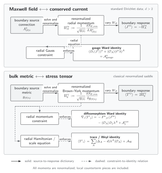
For standard Dirichlet data at a classical Euclidean AdS saddle, the leading boundary connection and metric are sources, while the finite renormalized radial momenta give the current and stress-tensor responses in the declared source convention. Solid arrows show the source-to-response dictionary. Dashed arrows show how the radial Gauss, momentum, and Hamiltonian equations enforce the gauge, diffeomorphism, and trace or Weyl Ward identities. Local counterterm pieces and possible anomalies are retained. The diagram is schematic and not to scale.

The table is the diagram’s text-equivalent map and supports direct comparison of the same relations. On a narrow screen, scroll horizontally without shrinking the text.

Radial data and constraints in the current and stress-tensor dictionary

Boundary datum	Finite radial response	Bulk constraint	Boundary identity
Connection A(0)ia	Renormalized Maxwell momentum; gives ⟨Jia⟩	Gauss constraint	Gauge Ward identity, including charged sources and any gauge anomaly
Metric g(0)ij	Renormalized Brown–York momentum; gives ⟨Tij⟩	Momentum constraint	Diffeomorphism Ward identity, including work done by background sources
Weyl rescaling of the metric source g(0)ij	Trace of the metric response	Radial Hamiltonian equation and logarithmic terms	Trace identity, explicit source breaking, and Weyl anomaly

What normalization changes can and cannot do

Several operations that look like “rescaling a field” have different physical content. On a narrow screen, scroll horizontally without shrinking the text.

Adversarial normalization tests

Operation	What changes	What must still be checked
Multiply the Maxwell action by q at fixed A(0)	The nonlocal saddle functional and CJ both multiply by q	The old coefficient cannot be retained; positivity requires q > 0
Change current basis, J′ = rJ, A′(0) = A(0)/r	The pairing is unchanged while C′J = r2CJ	Generator normalization, charges, and the bulk coupling must be translated together
Add a finite local source counterterm	Contact terms and local curved-background responses	Separated-point CJ and CT remain fixed
Improve the stress tensor with an allowed dimension-(d − 2) scalar	The conformal-primary stress tensor and possibly its separated-point two-point coefficient	Translation Ward normalization, tracelessness, and operator mixing must be solved anew
Change the admissible gauge-field boundary condition	The boundary theory and which combination is source or response	The new variational problem, symplectic flux, global form, and charge lattice

The first row is a useful adversarial test. If $S_{E,A}\mapsto qS_{E,A}$ while $A_{(0)}$ is held fixed, then the radial momentum, $\langle J\rangle$, $W_{E,A}^{(2)}$, and $C_J$ all multiply by $q$. No source-local counterterm can restore the old separated-point coefficient. For $q<0$, $C_J<0$: reflection positivity fails and the bulk vector is a ghost. The graviton calculation has the analogous test, with a positive massless-graviton kinetic coefficient required for $C_T>0$.

Omitting the Gibbons–Hawking term is a different failure: normal derivatives of $\delta g$ remain, so the Dirichlet metric variational problem and the advertised stress response are not defined. Omitting or changing a finite curvature counterterm instead changes only local/contact data. These failures must not be conflated.

Domain of the result and where to continue

The exact coefficients above assume a classical saddle about Euclidean AdS, standard Dirichlet sources, the displayed component Maxwell normalization, a nondegenerate massless graviton, $d>2$, and separated boundary points. Bulk loops correct the saddle expansion. Higher derivatives can change effective kinetic coefficients and introduce additional modes. Logarithms, anomalies, parity-odd contact terms, charged sources, and nontrivial backgrounds require the full renormalized action rather than the flat-source formulas alone.

In AdS$_4$, electric, magnetic, or mixed gauge-field boundary conditions can turn a boundary global symmetry into a dynamical gauge field. For an Abelian $U(1)$ sector with properly quantized charges and contact terms and a chosen spin structure, these operations generate the familiar $SL(2,\mathbb Z)$ action. Without a spin structure, only the subgroup generated by $S$ and $T^2$ is always defined Witten 2003, §§2–3 and 5, especially printed p. 3, Open PDF. This is a change of boundary theory, not a finite counterterm Marolf and Ross 2006, §§4.1–4.4, printed pp. 12–18, Open PDF. Mixed gravitational boundary conditions can likewise make the boundary metric dynamical and lie outside the fixed-$g_{(0)}$ calculation Compère and Marolf 2008, §§2–3, Open PDF. Boundary Global Symmetry, Bulk Gauge Symmetry, and Global Form adds bundles, charge lattices, and global form that local two-point functions cannot determine. Renormalized One-Point Functions develops finite Brown–York and matter responses in general backgrounds. Central Charge, Newton Coupling, and the Planck Scale explains what a large $C_T$ does—and does not—establish about a semiclassical bulk.

Common pitfalls

Mixing Lorentzian and Euclidean signs mid-calculation. Wick rotate the action and declare the source variation before reading a response. A correct radial coefficient with the wrong $W_E$ sign gives the wrong operator convention.

Comparing $C_J$ without a generator basis. The component action, invariant metric, source, current, and charge lattice form one normalization package. A bare number called $C_J$ is not basis independent.

Calling every local term an anomaly. Finite local counterterms shift contact terms and cohomologically trivial pieces. A genuine gauge or Weyl anomaly is an obstruction that cannot be removed by an allowed invariant counterterm.

Treating the metric like a freely rescalable scalar source. The translation Ward identity fixes the physical stress tensor. In higher-curvature gravity, identify the massless transverse-traceless kinetic coefficient instead of silently replacing it by a bare Newton constant.

Inferring global symmetry data from the Gauss constraint. The local Ward identity does not determine the global form of the group, allowed bundles, line operators, or charge lattice.

Exercises

1. Derive the gauge Ward identity

Take $\delta_\alpha A_{(0)i}^a=(D_i\alpha)^a$ and $\delta_\alpha\lambda^A=-\alpha^a(t^a\lambda)^A$. Use the source variation to derive the anomaly-free identity.

Solution — gauge variation

Substitution gives

$$\delta_\alpha W_E =\int\sqrt{g_{(0)}}\left[ \langle J^{ia}\rangle(D_i\alpha)^a -\alpha^a\langle\mathcal O_A\rangle(t^a\lambda)^A \right].$$

Integrating the first term by parts and requiring $\delta_\alpha W_E=0$ for arbitrary $\alpha^a$ gives

$$(D_i\langle J^i\rangle)^a +\langle\mathcal O_A\rangle(t^a\lambda)^A=0.$$

If the functional has a gauge anomaly, $\delta_\alpha W_E=-\int\sqrt{g_{(0)}}\,\alpha^a\mathcal A_{\mathrm{gauge}}^a$ supplies the displayed right-hand side.

2. Derive the metric Ward identities

Use the gauge-covariant diffeomorphism variations

$$\delta_\xi g_{(0)ij}=2\nabla_{(i}\xi_{j)}, \qquad \delta_\xi A_{(0)i}^a=\xi^kF^a_{ki}, \qquad \delta_\xi\lambda^A=\xi^kD_k\lambda^A$$

to derive the diffeomorphism Ward identity. Then derive the trace identity from

$$\delta_\sigma g_{(0)ij}=2\sigma g_{(0)ij}, \qquad \delta_\sigma A_{(0)i}^a=0, \qquad \delta_\sigma\lambda^A=(\Delta_A-d)\sigma\lambda^A.$$

Solution — diffeomorphism and Weyl variations

The gauge-covariant diffeomorphism gives

$$\begin{aligned} \delta_\xi^{\mathrm{cov}}W_E =\int\sqrt{g_{(0)}}\bigl[ &\langle J^{ia}\rangle\xi^kF^a_{ki} +\langle\mathcal O_A\rangle\xi^kD_k\lambda^A\\ &-\langle T^{ij}\rangle\nabla_i\xi_j \bigr]. \end{aligned}$$

The last sign comes from $-\tfrac12\langle T^{ij}\rangle\delta g_{(0)ij}$ and the symmetry of $T^{ij}$. Integrating it by parts and relabeling the free index gives

$$\delta_\xi^{\mathrm{cov}}W_E =\int\sqrt{g_{(0)}}\,\xi^j\left[ \nabla_i\langle T^i{}_j\rangle +F^a{}_{ji}\langle J^{ia}\rangle +\langle\mathcal O_A\rangle D_j\lambda^A \right].$$

Equating this to $\int\sqrt{g_{(0)}}\,\xi^j\mathcal A_j^{\mathrm{cov}}$ yields

$$\nabla_i\langle T^i{}_j\rangle =-F^a{}_{ji}\langle J^{ia}\rangle -\langle\mathcal O_A\rangle D_j\lambda^A +\mathcal A_j^{\mathrm{cov}}.$$

For a Weyl variation, $\delta_\sigma A_{(0)}=0$ and the other source variations give

$$\delta_\sigma W_E =\int\sqrt{g_{(0)}}\,\sigma\left[ \sum_A(\Delta_A-d)\lambda^A\langle\mathcal O_A\rangle -\langle T^i{}_i\rangle \right].$$

Using $\delta_\sigma W_E=-\int\sqrt{g_{(0)}}\,\sigma\mathcal A_{\mathrm W}$ therefore gives

$$\langle T^i{}_i\rangle =\sum_A(\Delta_A-d)\lambda^A\langle\mathcal O_A\rangle +\mathcal A_{\mathrm W}.$$

3. Check transversality away from contact points

Show directly that

$$\partial_i\left[ \frac{I_{ij}(x)}{(x^2)^{d-1}} \right]=0, \qquad x\neq0.$$

Solution — transverse current kernel

Write $r^2=x^2$. The derivative of the first term is

$$\partial_i\left(\delta_{ij}r^{-2d+2}\right) =-2(d-1)x_jr^{-2d}.$$

For the second term,

$$\partial_i\left(x_ix_jr^{-2d}\right) =(1-d)x_jr^{-2d},$$

so multiplying it by $-2$ gives $+2(d-1)x_jr^{-2d}$. The pieces cancel for $x\neq0$. At $x=0$, the distributional extension contains the contact terms required by the Ward identity.

4. Perform the AdS₅/CFT₄ coefficient check

Insert $d=4$ into the general $C_J$ and $C_T$ formulas. Then use $C_T=40c/\pi^4$ to solve for $c$ in two-derivative Einstein gravity.

Solution — four-dimensional coefficients

Since $\Gamma(4)=6$, $\Gamma(5)=24$, and $\Gamma(2)=1$,

$$C_J =\frac{2\cdot6}{2\pi^2}\frac{L}{g_5^2} =\frac{6L}{\pi^2g_5^2},$$

and

$$C_T =\frac53\frac{24}{\pi^2} \frac{L^3}{8\pi G_5} =\frac{5L^3}{\pi^3G_5}.$$

Equating the latter to $40c/\pi^4$ yields

$$c=\frac{\pi L^3}{8G_5}.$$

The two sides use different standard meanings of “central charge,” so the conversion factor is essential.

5. Separate a kinetic rescaling from a basis change

First multiply $S_{E,A}$ by $q>0$ while holding $A_{(0)}$ fixed. Then instead make the basis change $J'=rJ$ and $A'_{(0)}=A_{(0)}/r$. How does the reported current coefficient change in each case?

Solution — two inequivalent rescalings

At fixed source, the radial momentum and the nonlocal quadratic functional scale by $q$, so two source derivatives give

$$C_J\longmapsto qC_J.$$

This is a physical change of the kinetic normalization. For the basis change,

$$\int A'_{(0)}J'=\int A_{(0)}J,$$

but $\langle J'J'\rangle=r^2\langle JJ\rangle$, so

$$C'_J=r^2C_J.$$

The second change is a relabeling only if the generators, charges, and bulk field normalization are translated with it. The equality of source pairings distinguishes it from the fixed-source kinetic rescaling.

The chapter overview contains the structure diagram and validity and failure diagram. They are embedded there once so that their shared chapter-level context is not repeated on every article.

For the chapter-wide comparison of assumptions, counterevidence, falsifiers, and claim ceilings, see the claim-domain table.

References

• Bardeen, William A., and Bruno Zumino. “Consistent and Covariant Anomalies in Gauge and Gravitational Theories.” Nuclear Physics B 244 (1984): 421–453. DOI. Open PDF.
• Bianchi, Massimo, Daniel Z. Freedman, and Kostas Skenderis. “Holographic Renormalization.” Nuclear Physics B 631 (2002): 159–194. DOI. Open PDF.
• Buchel, Alex, Jorge Escobedo, Robert C. Myers, Miguel F. Paulos, Aninda Sinha, and Michael Smolkin. “Holographic GB Gravity in Arbitrary Dimensions.” Journal of High Energy Physics 2010 (3): 111. DOI. Open PDF.
• Compère, Geoffrey, and Donald Marolf. “Setting the Boundary Free in AdS/CFT.” Classical and Quantum Gravity 25 (2008): 195014. DOI. Open PDF.
• de Haro, Sebastian, Kostas Skenderis, and Sergey N. Solodukhin. “Holographic Reconstruction of Spacetime and Renormalization in the AdS/CFT Correspondence.” Communications in Mathematical Physics 217 (2001): 595–622. DOI. Open PDF.
• Freedman, Daniel Z., Samir D. Mathur, Alec Matusis, and Leonardo Rastelli. “Correlation Functions in the CFT$_d$/AdS$_{d+1}$ Correspondence.” Nuclear Physics B 546 (1999): 96–118. DOI. Open PDF.
• Henningson, Måns, and Kostas Skenderis. “The Holographic Weyl Anomaly.” Journal of High Energy Physics 1998 (7): 023. DOI. Open PDF.
• Marolf, Donald, and Simon F. Ross. “Boundary Conditions and Dualities: Vector Fields in AdS/CFT.” Journal of High Energy Physics 2006 (11): 085. DOI. Open PDF.
• Martelli, Dario, and Wolfgang Mück. “Holographic Renormalization and Ward Identities with the Hamilton–Jacobi Method.” Nuclear Physics B 654 (2003): 248–276. DOI. Open PDF.
• Mück, Wolfgang, and K. S. Viswanathan. “The Graviton in the AdS-CFT Correspondence: Solution via the Dirichlet Boundary Value Problem.” arXiv:hep-th/9810151 (1998). Open PDF.
• Osborn, Hugh, and Andreas C. Petkou. “Implications of Conformal Invariance in Field Theories for General Dimensions.” Annals of Physics 231 (1994): 311–362. DOI. Open PDF.
• Witten, Edward. “Anti-de Sitter Space and Holography.” Advances in Theoretical and Mathematical Physics 2 (1998): 253–291. DOI. Open PDF.
• Witten, Edward. “SL(2,$\mathbb Z$) Action on Three-Dimensional Conformal Field Theories with Abelian Symmetry.” In From Fields to Strings: Circumnavigating Theoretical Physics, vol. 2, edited by Mikhail Shifman et al., 1173–1200. Singapore: World Scientific, 2005. DOI. Open PDF.