BKL, Mixmaster, and Inhomogeneous Singularities

The Belinskii–Khalatnikov–Lifshitz (BKL) picture is a proposed local description of a spacelike singularity, not a theorem about every solution of Einstein’s equations. At a typical spatial point it predicts long, nearly Kasner intervals separated by short curvature-driven transitions. Bianchi IX, or Mixmaster, dynamics is the homogeneous laboratory for those transitions. Its lesson for quantum cosmology is sharp: a bounce of one isotropic scale factor does not control shear, curvature-wall scattering, spatial gradients, or spikes. Research-status statements on this page are checked through 30 August 2026.

Required background. Quantum-Cosmology Observables and the Problem of Time supplies the distinction between a coordinate evolution and a physical relational claim.

Helpful background. Higher-Derivative Semiclassical Initial-Value Problems, Renormalized Stress and Backreaction in FLRW, and Minisuperspace Reductions and Approximation Control supply comparison and truncation controls.

Kasner epochs and Mixmaster transitions

A Kasner epoch is an interval during which curvature terms are negligible and the metric at one spatial point is well approximated by a vacuum Bianchi I solution. In the site’s $(+---)$ convention,

$$ds^2=dt^2-\sum_{i=1}^{3}t^{2p_i}dx_i^2, \qquad \sum_i p_i=1, \qquad \sum_i p_i^2=1.$$

Except at special endpoints, one exponent is negative and two are positive: as $t\to0^+$, one principal direction expands while the local three-volume $a_1a_2a_3=t$ collapses.

One number, plus an axis ordering

Order the exponents as $p_{(1)}\le p_{(2)}\le p_{(3)}$ and define $u\in[1,\infty]$. Then

$$D(u)=1+u+u^2, \qquad p_{(1)}=-\frac{u}{D}, \qquad p_{(2)}=\frac{1+u}{D}, \qquad p_{(3)}=\frac{u(1+u)}{D}.$$

These expressions obey both Kasner constraints. The value $u=1$ gives the locally rotationally symmetric point $(-1/3,2/3,2/3)$, while $u=\infty$ denotes the Taub limit $(0,0,1)$. A value of $u$ alone suppresses the six possible assignments of the ordered exponents to the three spatial axes. Any calculation of successive collisions must therefore retain the axis permutation as well as $u$ Heinzle and Uggla 2009, §3, Eqs. (15)–(17).

A single Bianchi II curvature wall gives the transition law. If the incoming labels are chosen so that $p_1<0$, then before reordering the outgoing exponents are

$$\widetilde p_1=-\frac{p_1}{1+2p_1}, \qquad \widetilde p_2=\frac{p_2+2p_1}{1+2p_1}, \qquad \widetilde p_3=\frac{p_3+2p_1}{1+2p_1}.$$

Reordering the three outgoing exponents induces the Kasner map

$$T(u)= \begin{cases} u-1, & u\ge 2,\\[2pt] (u-1)^{-1}, & 1<u<2. \end{cases}$$

At $u=2$ the first branch reaches $u=1$; the ideal recursion then encounters a special endpoint. Rational initial values terminate in this exact discrete model, although nearby irrational values do not. The map and the full axis transition follow from the Bianchi I and II invariant subsets of the Bianchi IX system Heinzle and Uggla 2009, §5, Eqs. (22)–(23).

Epochs, eras, and what “chaos” means

An epoch is one nearly constant Kasner state. An era is the maximal run of subtraction steps. If an era begins at

$$\mathsf u_s=k_s+x_s, \qquad k_s=\lfloor\mathsf u_s\rfloor, \qquad 0<x_s<1,$$

then it contains $k_s$ epochs,

$$\mathsf u_s,\ \mathsf u_s-1,\ \ldots,\ 1+x_s,$$

and the next era begins at

$$\mathsf u_{s+1}=\frac{1}{x_s} =\frac{1}{\{\mathsf u_s\}}.$$

Thus a continued fraction $\mathsf u_s=[k_s;k_{s+1},k_{s+2},\ldots]$ loses its first entry after one era. This shift supplies exact symbolic and statistical results for the discrete map Heinzle and Uggla 2009, §5, Eqs. (24)–(28).

That fact must not be silently promoted into a theorem about every Bianchi IX orbit. After the logarithmic volume direction is projected out, the sharp-wall approximation gives a finite-volume billiard in the hyperbolic plane, whose generic geodesics have infinitely many collisions and strong chaotic features Damour, Henneaux, and Nicolai 2003, §§1.3 and 5.2.2. Ringström’s theorem proves that generic homogeneous Bianchi IX solutions approach the closure of the vacuum Bianchi I and II attractor. It does not prove that an arbitrary orbit shadows a prescribed infinite Kasner sequence, nor does it transfer the result to unrestricted inhomogeneous $3+1$ gravity Ringström 2001, §1, Eq. (1.9), pp. 5–7; Heinzle and Uggla 2009, §6, Theorem 6.1 and Eqs. (32)–(33). Misner’s original Mixmaster analysis is the historical source for treating Bianchi IX as a laboratory for this oscillatory approach Misner 1969, pp. 1071–1074.

Application: what isotropy discards

The following diagonal vacuum Bianchi IX calculation makes the discarded terms explicit. It is a homogeneous classical benchmark, not a model of a quantum bounce and not evidence for the generic inhomogeneous BKL conjecture.

Misner variables and the complete potential

Let $\sigma_i$ be left-invariant one-forms on $S^3$ normalized by

$$d\sigma_i=\frac12\epsilon_{ijk}\sigma_j\wedge\sigma_k,$$

and write

$$ds^2=N^2dt^2-\sum_{i=1}^{3}a_i^2\sigma_i^2, \qquad e^\alpha=(a_1a_2a_3)^{1/3}.$$

The anisotropy variables $\beta_\pm$ are defined by

$$\begin{aligned} a_1&=e^{\alpha+\beta_++\sqrt3\,\beta_-},\\ a_2&=e^{\alpha+\beta_+-\sqrt3\,\beta_-},\\ a_3&=e^{\alpha-2\beta_+}. \end{aligned}$$

The singular direction is decreasing $\alpha$. After fixed fiducial-volume and gravitational factors have been absorbed into the lapse and momenta, one convenient Hamiltonian constraint is

$$C=\frac12e^{-3\alpha} \left(-p_\alpha^2+p_+^2+p_-^2\right) +e^\alpha V(\beta_+,\beta_-)=0,$$

with the full Bianchi IX potential

$$\begin{aligned} V(\beta_+,\beta_-)=\frac16\big[&e^{-8\beta_+} +2e^{4\beta_+}\big(\cosh(4\sqrt3\,\beta_-)-1\big)\\ &-4e^{-2\beta_+}\cosh(2\sqrt3\,\beta_-)\big]. \end{aligned}$$

The overall positive normalization of $C$ is lapse-dependent; the displayed relative signs and exponential powers are not. Bojowald, Brizuela, Calizaya Cabrera, and Uria give this one-form, variable, constraint, and potential convention using the opposite metric signature; reversing the displayed line-element signature and making the corresponding overall canonical convention choice leaves the constraint surface and reduced equations written here unchanged Bojowald et al. 2024, §II, Eqs. (1)–(6), pp. 2–3.

Choose the constraint sheet $p_\alpha=-\mathcal H$ and use $\alpha$ as the evolution parameter. The reduced Hamiltonian and equations are

$$\mathcal H=\sqrt{p_+^2+p_-^2+2e^{4\alpha}V},$$ $$\beta_\pm'=\frac{p_\pm}{\mathcal H}, \qquad p_\pm'=-\frac{e^{4\alpha}}{\mathcal H} \frac{\partial V}{\partial\beta_\pm}, \qquad '\equiv\frac{d}{d\alpha}.$$

On the sheet $p_\alpha=-\mathcal H$, integrating toward smaller $\alpha$ follows an expanding solution backward toward its singularity. The sheet $p_\alpha=+\mathcal H$ follows the time-reversed contracting solution forward and traces the same configuration-space path. These reduced equations are Bojowald et al. 2024, §II, Eqs. (7)–(11), pp. 3–4.

During a kinetic interval, the three axis exponents can be read directly from the numerical slopes:

$$\begin{aligned} p_1&=\frac{1+\beta_+'+\sqrt3\,\beta_-'}{3},\\ p_2&=\frac{1+\beta_+'-\sqrt3\,\beta_-'}{3},\\ p_3&=\frac{1-2\beta_+'}{3}. \end{aligned}$$

After sorting, the measured parameter is $u=p_{(3)}/p_{(2)}$. Two dimensionless diagnostics identify a kinetic window:

$$R_V=\frac{\lvert2e^{4\alpha}V\rvert}{p_+^2+p_-^2}, \qquad R_F=\frac{e^{4\alpha}\sqrt{(\partial_+V)^2+(\partial_-V)^2}} {p_+^2+p_-^2}.$$

Small $R_V$ checks that the Hamiltonian is kinetically dominated; small $R_F$ checks that the momenta are nearly constant. Neither criterion should be inferred from a visually straight segment alone.

Reproducible trajectory and two wall encounters

The fixture starts at

$$(\alpha,\beta_+,\beta_-,p_+,p_-) =(-5,0,0,-143,-95\sqrt3)$$

and integrates to $\alpha=-50$ with fixed-step fourth-order Runge–Kutta. The production step is $\Delta\alpha=-5\times10^{-4}$; a second run uses half that step. At the finite initial point, $V(0,0)=-1/2$ is exponentially suppressed but not zero. After neglecting that wall term—the exact zero-wall, kinetic-limit fixture—the ordered exponents are

$$\left(-\frac{35}{109},\frac{60}{109},\frac{84}{109}\right), \qquad u_0=\frac75.$$

The map predicts both branches,

$$\frac75\xrightarrow{\text{invert}}\frac52 \xrightarrow{\text{subtract}}\frac32.$$

The measured kinetic windows are:

Epoch	$\alpha$	Ordered $(p_{(1)},p_{(2)},p_{(3)})$	Measured $u$	Map prediction	Map residual	$R_V$
0	$-8$	$(-0.321100917,\ 0.550458715,\ 0.770642202)$	$1.40000000057$	—	—	$1.51\times10^{-9}$
1	$-20$	$(-0.256410256,\ 0.358974359,\ 0.897435897)$	$2.50000000000$	$2.49999999643$	$3.57\times10^{-9}$	$1.06\times10^{-28}$
2	$-48$	$(-0.315789474,\ 0.526315789,\ 0.789473684)$	$1.50000000000$	$1.50000000000$	$3.58\times10^{-13}$	$6.35\times10^{-20}$

The first and second wall-ratio maxima occur at $\alpha=-13.3700$ and $-40.8585$, with peak $R_V=6.3802$ and $0.68027$. The following deterministic diagnostics test resolution and algebraic identities; they do not bound model error or the total numerical error:

Check over the recorded run	Maximum
Change in plateau $u$ after halving the step	$9.10\times10^{-13}$
Shift of a collision location after halving the step	$2.50\times10^{-4}$ in $\alpha$
Kasner-square residual in the three selected windows	$1.01\times10^{-9}$
Reconstructed-constraint floating-point residual	$8.61\times10^{-17}$
Scaled potential-invariance residual under the $120^\circ$ rotation	$8.70\times10^{-16}$
Scaled gradient-covariance residual under the same rotation	$8.08\times10^{-16}$
Scaled residual of applying the rotation three times	$5.55\times10^{-17}$

The reconstructed-constraint number is an algebraic consistency check because $p_\alpha$ was eliminated by the square root; it is not an independent conservation test. Step halving, the small values of $R_V$ and $R_F$ in the declared fixed windows, and the rotation and isotropic controls are the substantive implementation checks. The calculation is reproducible from the sampled trace, epoch summary, collision summary, control summary, and semantic record.

The left panel below shows the orbit in anisotropy space and locates the two wall encounters. The right panel gives the decisive comparison: the extracted plateaus follow the invert and subtract branches of the ideal Kasner map.

On a narrow screen, swipe or use the Left and Right arrow keys to pan across the figure. Home and End move to its edges. A full-size link is also available.

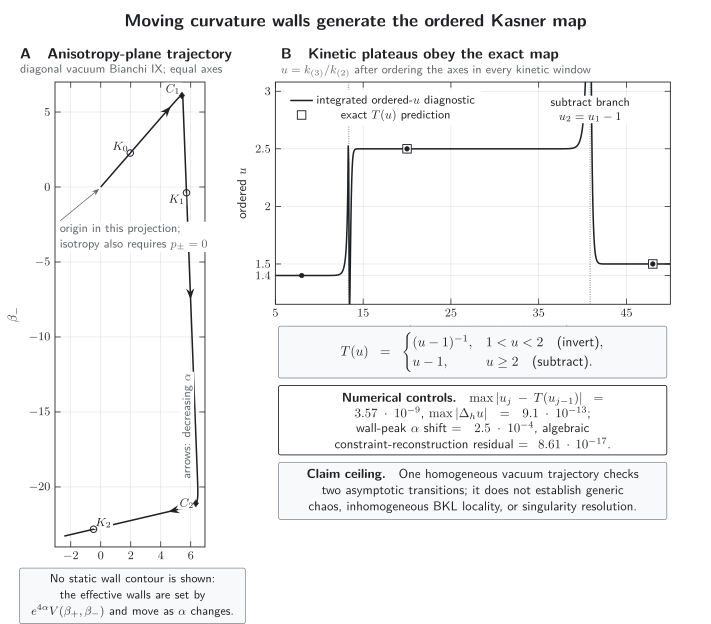
Quantitative homogeneous-vacuum benchmark. The trajectory uses the displayed Misner convention, initial data, and fixed-step integration. Two wall encounters connect kinetic plateaus with $u=7/5$, $5/2$, and $3/2$ within the residuals in the table. This one orbit checks the implementation and two Kasner transitions; it does not establish generic chaos, inhomogeneous BKL locality, quantum suppression, or singularity resolution.

The isotropic restriction is not “zero curvature”

Setting $\beta_+=\beta_-=p_+=p_-=0$ removes anisotropy motion and wall scattering, but

$$V(0,0)=-\frac12, \qquad \nabla_\beta V(0,0)=0.$$

The remaining value is the closed-FLRW spatial-curvature term. Moreover, in the vacuum model displayed above this formal restriction gives $\mathcal H^2=-e^{4\alpha}$, so it is not by itself a real constrained vacuum trajectory. A physical isotropic closed-FLRW comparison needs matter or a cosmological term. The honest comparison is therefore about discarded terms: isotropy deletes the two shape momenta and their anisotropy-dependent scattering, but it does not delete spatial curvature.

Shear and matter change the asymptotics

Let $a=(a_1a_2a_3)^{1/3}$ and define the shear scalar by

$$\sigma^2=\frac12\sigma^i{}_j\sigma^j{}_i.$$

In Bianchi I, when anisotropic stress is negligible,

$$\dot\sigma^i{}_j+3H\sigma^i{}_j=0 \quad\Longrightarrow\quad \sigma^i{}_j=\frac{\Sigma^i{}_j}{a^3}, \qquad \sigma^2\propto a^{-6}.$$

If an effective shear density is useful, define $\rho_\sigma=\sigma^2/(8\pi G)$; then the flat Bianchi I constraint is $3H^2=8\pi G\rho+\sigma^2$. For a perfect fluid with $p=w\rho$,

$$\rho_w\propto a^{-3(1+w)}, \qquad \frac{\rho_\sigma}{\rho_w}\propto a^{-3(1-w)}.$$

During contraction this gives three distinct regimes:

Matter	Relative behavior as $a\to0$	What follows
$w<1$	Shear grows faster	A small anisotropy can overtake the fluid
$w=1$	Shear and matter tie	Relative redshifting alone suppresses neither
$w>1$	Matter grows faster	Ekpyrotic matter suppresses shear relative to its own density

A canonical massless scalar is the subtle middle case. For

$$\phi=q\ln t+\phi_0,$$

the generalized Kasner relations are

$$\sum_i p_i=1, \qquad \sum_i p_i^2+8\pi Gq^2=1.$$

Unlike the vacuum circle, this system has an open region with all three $p_i>0$. Curvature walls then recede too quickly to cause an endless sequence of collisions; homogeneous stiff-fluid Bianchi class A solutions approach one limiting point Ringström 2001, §1, pp. 1–2, and §7. This is a change in Kasner stability, not dilution of shear. Rigorous inhomogeneous Einstein–scalar and stiff-fluid solutions with quiescent, velocity-dominated singularities are known for analytic asymptotic data with positive Kasner eigenvalues Andersson and Rendall 2001, §2.3, Theorems 2.1–2.2, and §8. Those existence theorems do not say that every smooth stiff-matter Cauchy datum approaches that class. Scalar potentials, tilt, anisotropic stress, and form fields can also change the wall system.

Ultralocality, gradients, and spikes

Ultralocal means that, asymptotically and at a generic spatial point, the leading evolution is approximated by ordinary differential equations in time. It does not mean that every spatial derivative is set to zero. In four-dimensional vacuum gravity, local spatial-curvature coefficients generate the dominant walls; subdominant gradient terms are expected to lose against the exponential wall hierarchy between collisions. The Hamiltonian and momentum constraints also continue to restrict the data Damour, Henneaux, and Nicolai 2003, §§5.4–5.5, Eqs. (5.38)–(5.42).

A fixed smooth-gradient check illustrates the pointwise competition without settling the nonlinear problem. On the canonical massless-scalar Kasner background $\phi=q\ln t+\phi_0$, suppose one comoving component $\partial_i\phi$ remains finite and nonzero. Its physical gradient energy scales as $\rho_{\nabla,i}\propto g^{ii}(\partial_i\phi)^2\propto t^{-2p_i}$, whereas the homogeneous kinetic energy scales as $\rho_{\mathrm{kin}}\propto t^{-2}$. Hence

$$\frac{\rho_{\nabla,i}}{\rho_{\mathrm{kin}}} \propto t^{2(1-p_i)}\longrightarrow0 \qquad (t\to0^+,\ p_i<1).$$

This is only an ordinary-worldline control for a fixed smooth gradient and a nondegenerate Kasner exponent. It is not uniform in space and is not, by itself, a constraint-compatible nonlinear Einstein–scalar solution. Exceptional locations can behave differently.

The difficult points are those at which the coefficient of a normally dominant transition vanishes. A local toy model makes the mechanism visible:

$$U_{\mathrm{wall}}(x,\beta)=c(x)^2e^{-2w(\beta)}, \qquad c(x)=\varepsilon x.$$

Every nearby timeline with $x\ne0$ encounters the wall, while the timeline at $x=0$ does not. The two histories acquire different Kasner labels, the spatial profile sharpens, and gradients can become leading in a shrinking neighborhood. This coefficient model is schematic, not an exact solution of the Einstein constraints. Exact vacuum $G_2$ solutions and their transition chains exhibit the corresponding spike mechanism Heinzle, Uggla, and Lim 2012, §§3–5.

This distinction defeats a common shortcut:

$$\text{pointwise convergence away from spikes} \qquad\not\Longrightarrow\qquad \text{uniform control of gradients or curvature maxima}.$$

A reproducible inhomogeneous adversary should therefore add a constraint-compatible mode with fixed comoving wave number and amplitude, not merely insert $c(x)$ into a homogeneous Hamiltonian. It should then vary phase and wave number, add further modes, refine spatial resolution, and monitor both averaged and spike-sensitive norms. One useful declared diagnostic is

$$\epsilon_\nabla(\tau)= \frac{\lVert\mathcal H_\nabla\rVert+\lVert\mathcal M_\nabla\rVert} {\lVert\mathcal H_{\mathrm{time}}\rVert+\lVert\mathcal M_{\mathrm{time}}\rVert},$$

where the Hamiltonian and momentum pieces, norm, gauge, domain, and any excluded shrinking spike neighborhoods must all be stated. A volume average alone can miss the failure.

Recent rigorous results strengthen selected parts of this picture without proving the unrestricted conjecture. In Gowdy symmetry, an open class of inhomogeneous vacuum data can exhibit a controlled BKL-like bounce, AVTD asymptotics, and spikes Li 2024, §§1.3–1.5 and Theorems 2.1–2.2. The result is symmetry-reduced and controls a finite bounce mechanism; the same work states multiple or infinite bounces beyond its regime as conjectures.

What is established, and in which domain?

The evidence hierarchy matters more than the word “generic.” Here generic is never used without its domain and exceptional set.

Domain	Strongest supported statement	What is not licensed
Exact Bianchi I/II	Kasner solutions and the single-wall transition map are exact	A generic Bianchi IX or inhomogeneous orbit
Homogeneous Bianchi IX	Outside specified exceptional asymptotically self-similar or Taub-type sets, the orbit approaches the vacuum I/II attractor	A prescribed infinite symbolic sequence or unrestricted $3+1$ behavior
Sharp-wall hyperbolic billiard	Finite volume gives generic repeated collisions and strong chaotic properties within the asymptotic billiard	Coordinate-independent chaos for the full Einstein flow without the limiting assumptions
Analytic Einstein–scalar/stiff families	Quiescent velocity-dominated singularities exist with the full functional degree count	Every smooth Cauchy datum, every matter coupling, or vacuum oscillatory BKL
Symmetry-reduced inhomogeneous systems	Exact spike chains, numerical evidence, and recent finite-bounce theorems support specific mechanisms	A theorem for unconstrained vacuum $3+1$ initial data
General vacuum $3+1$ gravity	BKL plus spike corrections is a well-developed conjectural asymptotic picture	Proven generic Mixmaster chaos, uniform ultralocality, or universal singularity structure

The original BKL analysis remains the historical source of the oscillatory local picture Belinskii, Khalatnikov, and Lifshitz 1970, pp. 525–573. The conjecture’s local and oscillatory content, its matter-dependent exceptions, and the limits of homogeneous Bianchi IX results are reviewed in Ringström 2025, §2.4, pp. 56–57, and §3.1.1, pp. 60–61. The fact–conjecture boundary is reviewed sharply in Heinzle and Uggla 2009, §§6–9, while the spike correction is formulated in Heinzle, Uggla, and Lim 2012, abstract and §§1, 6. As of the date above, no theorem combines all of these mechanisms for unrestricted $3+1$ vacuum data.

Targets for a quantum-cosmology claim

The classical benchmark tells us what a claimed quantum suppression must control. A convincing test must specify:

1. Anisotropic states and observables. Give the state class, physical inner product, operator domains, clock, and observables corresponding to $\beta_\pm$, $p_\pm$, shear, and directional expansion.
2. Constraint and covariance control. Show that the quantum or effective constraints close in the sector used to reconstruct spacetime; a modified wall potential alone is insufficient.
3. A classical-recovery window. Recover Bianchi II scattering and the ordered Kasner map, including axis permutations, where curvature is low and quantum fluctuations are controlled.
4. Matter dependence. Repeat the test for the actual matter Hamiltonian. A result for a free stiff scalar cannot be exported to a potential-dominated, tilted, or anisotropic source.
5. Inhomogeneous convergence. Use constraint-compatible modes, increase their number and spatial resolution, and bound nonlinear backreaction. One perturbation mode is a truncation test, not genericity.
6. Spike-sensitive diagnostics. Track local or supremum norms, curvature and tidal components, and shrinking exceptional neighborhoods in addition to averages.
7. Uncertainty and alternatives. Vary quantization, state, clock, regulator, wall-detection threshold, and numerical resolution. Record which conclusion changes.

An adversarial pair is especially useful: construct two anisotropic or inhomogeneous completions with identical isotropic bounce data but different wall suppression or spike growth. The isotropic data cannot distinguish them. The strongest defensible conclusion is therefore model- and state-specific stability or continuation over a declared mode band and interval. It is not generic singularity resolution until the discarded sectors converge and the relevant geometric observables pass their own tests. This claim ceiling complements Bounce and Singularity-Resolution Claims and leads into Quantum Geometrodynamics Beyond Minisuperspace.

Common pitfalls

Treating $u$ as a complete state. It records ordered exponents, not which exponent belongs to which axis. Retain the permutation through every transition.

Equating a stiff scalar with ekpyrotic suppression. Both shear and a free stiff scalar scale as $a^{-6}$. Only $w>1$ matter wins by relative redshifting; the $w=1$ quiescent mechanism instead enlarges the Kasner stability region.

Calling ultralocality homogeneity. The leading evolution may be local while its coefficients vary with position and the constraints still couple spatial data. Spikes are the sharp counterexample to uniform locality.

Using a numerical orbit as a proof of chaos. The fixture verifies two transitions and its own convergence. Chaos and genericity require separate invariant definitions and quantified domains.

Promoting a volume bounce to spacetime resolution. A nonzero isotropic volume does not bound shear, tidal curvature, gradients, or spike growth.

Exercises

1. Verify the Kasner parametrization

Show directly that the ordered $u$-parametrization obeys both vacuum Kasner constraints.

Solution

With $D=1+u+u^2$,

$$p_{(1)}+p_{(2)}+p_{(3)} =\frac{-u+(1+u)+u(1+u)}{D} =\frac{1+u+u^2}{D}=1.$$

For the squares,

$$\begin{aligned} D^2\sum_i p_{(i)}^2 &=u^2+(1+u)^2+u^2(1+u)^2\\ &=1+2u+3u^2+2u^3+u^4\\ &=(1+u+u^2)^2=D^2. \end{aligned}$$

Hence $\sum_i p_{(i)}^2=1$. For $1<u<\infty$, the first exponent is negative and the other two are positive.

2. Reproduce the two map branches

Starting from $u_0=7/5$, apply the ideal Kasner map twice and compute the ordered exponents at all three epochs.

Solution

Because $1<7/5<2$, the first step is inversion:

$$u_1=\frac{1}{7/5-1}=\frac52.$$

The next step is subtraction:

$$u_2=\frac52-1=\frac32.$$

Substitution in the parametrization gives

$$u_0=\frac75: \quad \left(-\frac{35}{109},\frac{60}{109},\frac{84}{109}\right),$$ $$u_1=\frac52: \quad \left(-\frac{10}{39},\frac{14}{39},\frac{35}{39}\right),$$ $$u_2=\frac32: \quad \left(-\frac{6}{19},\frac{10}{19},\frac{15}{19}\right).$$

These are the rational values approached by the three numerical plateaus.

3. Read eras from a continued fraction

Use $\sqrt{10}=[3;\overline{6}]$ to find the first two era lengths and list the first five epochs.

Solution

The first partial quotient is $3$, so the first era has three epochs:

$$\sqrt{10},\qquad \sqrt{10}-1,\qquad \sqrt{10}-2.$$

Its fractional part is $\sqrt{10}-3$. The next era begins at

$$\frac{1}{\sqrt{10}-3}=\sqrt{10}+3.$$

The continued-fraction shift exposes the next partial quotient $6$, so the second era has six epochs. The first five epochs overall are therefore

$$\sqrt{10}\to\sqrt{10}-1\to\sqrt{10}-2 \to\sqrt{10}+3\to\sqrt{10}+2.$$

4. Separate stiff and ekpyrotic suppression

Derive the scaling of $\rho_\sigma/\rho_w$ and explain what happens for $w=0$, $w=1$, and $w=3$. Then show that a scalar can admit the isotropic generalized Kasner point $p_i=1/3$.

Solution

Using $\rho_\sigma\propto a^{-6}$ and $\rho_w\propto a^{-3(1+w)}$,

$$\frac{\rho_\sigma}{\rho_w}\propto a^{-3(1-w)}.$$

As $a\to0$, the ratio diverges for dust ($w=0$), stays constant for stiff matter ($w=1$), and vanishes for $w=3$. Thus only the last case suppresses shear by relative redshifting.

For $p_1=p_2=p_3=1/3$, the first generalized Kasner relation holds and

$$\sum_i p_i^2=\frac13.$$

The second relation requires $8\pi Gq^2=2/3$, which is positive. The same isotropic point is impossible in vacuum because there $\sum_i p_i^2$ would have to equal $1$.

5. Design a failure test

Suppose a quantum model reproduces the three plateau values in the figure and gives a nonzero minimum isotropic volume. List four further checks needed before claiming generic singularity resolution, and explain why a spatial average is insufficient near a spike.

Solution

Any four of the following are essential: closure of the modified constraints; state, clock, inner-product, and operator-domain control; bounded shear and directional expansion on an open state set; recovery of the classical wall map at low curvature; mode-number and spatial-resolution convergence; nonlinear backreaction; matter-model variation; local curvature and tidal observables; and robustness under quantization choices.

A spike occupies a narrowing spatial region. Its contribution to a volume average may tend to zero even while a local gradient or curvature maximum grows without bound. One must therefore accompany averages with a declared local or supremum norm and demonstrate resolution convergence in the spike neighborhood.

The chapter overview contains the structure diagram and validity and failure diagram. They are embedded there once so that their shared chapter-level context is not repeated on every article.

For the chapter-wide comparison of assumptions, counterevidence, falsifiers, and claim ceilings, see the claim-domain table.

References

• Andersson, Lars, and Alan D. Rendall. “Quiescent Cosmological Singularities.” Communications in Mathematical Physics 218 (2001): 479–511. DOI. Open PDF.
• Belinskii, V. A., I. M. Khalatnikov, and E. M. Lifshitz. “Oscillatory Approach to a Singular Point in the Relativistic Cosmology.” Advances in Physics 19 (1970): 525–573. DOI.
• Bojowald, Martin, David Brizuela, Paula Calizaya Cabrera, and Sara F. Uria. “Chaotic Behavior of the Bianchi IX Model under the Influence of Quantum Effects.” Physical Review D 109 (2024): 044038. DOI. Official accepted PDF.
• Damour, Thibault, Marc Henneaux, and Hermann Nicolai. “Cosmological Billiards.” Classical and Quantum Gravity 20 (2003): R145–R200. DOI. Open PDF.
• Heinzle, J. Mark, and Claes Uggla. “Mixmaster: Fact and Belief.” Classical and Quantum Gravity 26 (2009): 075016. DOI. Open PDF.
• Heinzle, J. Mark, Claes Uggla, and Woei Chet Lim. “Spike Oscillations.” Physical Review D 86 (2012): 104049. DOI. Open PDF.
• Li, Warren. “BKL Bounces Outside Homogeneity: Gowdy Symmetric Spacetimes.” arXiv:2408.12427 [gr-qc] (2024). arXiv.
• Misner, Charles W. “Mixmaster Universe.” Physical Review Letters 22 (1969): 1071–1074. DOI.
• Ringström, Hans. “The Bianchi IX Attractor.” Annales Henri Poincaré 2 (2001): 405–500. DOI. Open PDF.
• Ringström, Hans. “Cosmology, the Big Bang and the BKL Conjecture.” Comptes Rendus. Mécanique 353 (2025): 53–78. DOI.