Quantum Geometrodynamics Beyond Minisuperspace

Quantum geometrodynamics assigns a wavefunctional $\Psi[h_{ab}(x),\varphi(x)]$ to spatial geometry and matter. Its configuration space is superspace—roughly, spatial metrics modulo spatial diffeomorphisms—not spacetime itself. Moving beyond minisuperspace means retaining genuine spatial dependence while preserving the constraints that separate physical geometry from coordinate redundancy.

For a fixed spatial manifold $\Sigma$, this quotient is written schematically as $\operatorname{Riem}(\Sigma)/\operatorname{Diff}(\Sigma)$. A minisuperspace keeps only finitely many symmetry-reduced coordinates; a mode truncation keeps selected spatial dependence; full superspace retains fields at every point.

The worked calculation on this page is deliberately narrower than a solution of the full functional theory. After the linearized constraints are solved in a gauge-invariant variable, one inhomogeneous perturbation mode can be coupled to one oscillatory WKB branch of a quantum background. A Born–Oppenheimer expansion then produces a branch-time Schrödinger equation and an explicit $m_{\mathrm P}^{-2}$ correction. The calculation is useful precisely because its regulator, clock, state, observable, and failure tests can all be displayed.

Required background. Wheeler–DeWitt Cosmology: Boundary Conditions, Inner Products, and Probabilities supplies WKB branches, superspace current, and the inner-product problem. BKL, Mixmaster, and Inhomogeneous Singularities shows what an exactly homogeneous truncation omits.

Helpful background. 2PI Effective Actions and Conserving Truncations separates a self-consistent closure from exact dynamics. Convergence, Extrapolation, and Error Certification supplies observable-level cutoff tests.

Reading path. The first two sections explain what is lost when the functional theory is reduced to one mode. Readers focused on the calculation can then follow the Born–Oppenheimer hierarchy and de Sitter benchmark; readers evaluating a claimed prediction should continue through the control record and adversarial mode-addition test.

Four local constraint densities at every spatial point

On a spatial slice $\Sigma$, the canonical variables are a positive-definite metric $h_{ab}(x)$ and its momentum $\pi^{ab}(x)$, together with matter fields. Write $h=\det h_{ab}$ and $\pi=h_{ab}\pi^{ab}$; $D_a$ is the derivative compatible with $h_{ab}$. For a scalar field $\varphi$ with conjugate momentum $\pi_\varphi$, there is one Hamiltonian-constraint density and three momentum-constraint densities at every point $x$:

$$\begin{aligned} \mathcal H_\perp &=\frac{16\pi G}{\sqrt h} \left(\pi^{ab}\pi_{ab}-\frac12\pi^2\right) -\frac{\sqrt h}{16\pi G} \left({}^{(3)}R-2\Lambda\right) +\mathcal H_\perp^{\mathrm m}\approx0,\\ \mathcal H_a &=-2D_b\pi^b{}_a+\pi_\varphi\,\partial_a\varphi\approx0. \end{aligned}$$

Here ${}^{(3)}R$ is the scalar curvature of $h_{ab}$, $\Lambda$ is the cosmological constant, and $\mathcal H_\perp^{\mathrm m}$ is the matter contribution to the Hamiltonian-constraint density.

The gravitational kinetic term is the quadratic form defined by the DeWitt supermetric,

$$G_{abcd}(x) =\frac{1}{2\sqrt h} \left(h_{ac}h_{bd}+h_{ad}h_{bc}-h_{ab}h_{cd}\right),$$

since $G_{abcd}\pi^{ab}\pi^{cd}=h^{-1/2}(\pi^{ab}\pi_{ab}-\pi^2/2)$. Its negative conformal direction is why the Wheeler–DeWitt equation resembles a Klein–Gordon equation on configuration space rather than an ordinary stationary Schrödinger equation.

The first relation generates normal deformations of $\Sigma$; the three components of the second generate spatial diffeomorphisms. Smearing them with a lapse $N$ and shift $N^a$ gives $H[N]$ and $D[\mathbf N]$. Their Poisson brackets are not four independent copies of an ordinary Lie algebra:

$$\begin{aligned} \{D[\mathbf N],D[\mathbf M]\} &=D[[\mathbf N,\mathbf M]],\\ \{D[\mathbf N],H[M]\} &=H[\mathcal L_{\mathbf N}M],\\ \{H[N],H[M]\} &=D[\boldsymbol\beta], \qquad \beta^a=h^{ab}(N\partial_bM-M\partial_bN). \end{aligned}$$

The metric in $\boldsymbol\beta$ is itself dynamical. These structure functions encode the fact that two successive changes of slicing differ by a spatial diffeomorphism. Teitelboim derives the three displayed brackets geometrically and shows how path independence of hypersurface evolution supplies the closure condition Teitelboim 1973, Eqs. (6a–c), pp. 545–546; Eq. (14), pp. 549–550. They are therefore part of the physics to be recovered, not optional bookkeeping.

The geometric meaning and sign conventions of this algebra are developed on Canonical Constraints, Dirac Observables, and Constraint Algebras. Here it is the consistency target for the quantum truncation.

Dirac quantization asks for

$$\widehat{\mathcal H}_\perp(x)\Psi=0, \qquad \widehat{\mathcal H}_a(x)\Psi=0.$$

At coincident points, the kinetic term contains products of functional derivatives. A regulator, factor ordering, operator domain, and removal of the regulator must therefore be specified before the first equation is an operator rather than a symbol. Different formal evaluations can give different commutators, and fixed-background point splitting generally has no well-defined coincidence limit Friedman and Jack 1988, §§ II–IV, pp. 3495–3504. A candidate quantization must also control

$$[\widehat H[N],\widehat H[M]] =i\widehat D[\boldsymbol\beta] +\widehat{\mathcal A}[N,M],$$

where the anomaly $\widehat{\mathcal A}$ must vanish in the claimed continuum theory or be shown to be a controlled deformation. A finite lattice can make this question explicit, but a computed lattice algebra and a kinematical representation of positive-definite metrics do not by themselves establish a continuum physical Hilbert space Lang and Schander 2024a, §§ 2–6; Lang and Schander 2024b, §§ 2–5.

A one-mode reduction makes the approximations explicit

This restores one linear inhomogeneous degree of freedom around FLRW. It still omits the nonlinear anisotropic-curvature walls, mode coupling, and spike dynamics exhibited by the preceding BKL analysis.

Consider a spatially flat FLRW background with a scalar inflaton. Put the system in a fiducial comoving box so that momenta are discrete, and define

$$\alpha=\ln(a/a_0), \qquad m_{\mathrm P}^2=\frac{3}{4\pi G}=6M_{\mathrm{Pl}}^2, \qquad \widetilde\phi=\frac{\phi}{m_{\mathrm P}}.$$

Here $a_0$ is a fixed reference value of the scale factor, with the same length dimension as $a$, and $M_{\mathrm{Pl}}=(8\pi G)^{-1/2}$ is the reduced Planck mass. The rescaled $m_{\mathrm P}$ is used only to match the explicit expansion below. The fiducial box is a normalization device; a final dimensionless observable must not depend on it.

Finite-box conventions and dimensions

The finite-box convention matters for dimensional consistency. Let $\mathfrak L$ be the fixed reference length used to normalize the comoving box, so $[\mathfrak L]=L$. Starting from the usual dimensionful conformal coordinates, the cited calculation rescales

$$a_{\mathrm{new}}=\mathfrak L a_{\mathrm{old}}, \qquad \eta_{\mathrm{new}}=\frac{\eta_{\mathrm{old}}}{\mathfrak L}, \qquad (v_{\mathbf k})_{\mathrm{new}} =\frac{(v_{\mathbf k})_{\mathrm{old}}}{\mathfrak L^2}, \qquad k_{\mathrm{new}}=\mathfrak L k_{\mathrm{old}}.$$

In units $c=\hbar=1$, $a$ and $a_0$ then have dimensions of length, whereas $\eta$, $k$, $v_k$, and $\widehat{\mathcal H}_k$ are dimensionless. Keeping $a_0$ explicit below prevents the shorthand $a_0=1$ from hiding powers of length Brizuela, Kiefer, and Krämer 2016a, § III.A–B, Eqs. (35), (51), and (53)–(57).

Solve the linearized constraints first

At quadratic order, the scalar metric and inflaton perturbations can be combined into the gauge-invariant Mukhanov–Sasaki variable $v$. A tensor polarization has the same oscillator form. For one real component of the $(\mathbf k,-\mathbf k)$ pair,

$$\widehat{\mathcal H}_k =\frac12\left[-\partial_{v_k}^2 +\omega_k^2(\eta)v_k^2\right],$$

with

$${}^{\mathrm S}\omega_k^2=k^2-\frac{z''}{z}, \qquad {}^{\mathrm T}\omega_k^2=k^2-\frac{a''}{a}, \qquad z=\frac{a\phi'}{\mathcal H}, \quad \mathcal H=\frac{a'}a.$$

Primes denote conformal-time derivatives. In the reduced quadratic action, the lapse and shift constraints have already been solved, and the remaining physical scalar degree of freedom can be represented by the gauge-invariant variable $v_k$. Gauge invariance is the result of that canonical reduction, not by itself a proof that the constraints were solved. The reduction is a major simplification—and also the reason this model cannot test the full nonlinear quantum constraint algebra.

The reduction and Fourier normalization are derived on Mukhanov–Sasaki Scalar Modes. The present calculation imports that physical oscillator and asks what changes when its background is also quantized.

Treating homogeneous background variables nonperturbatively while retaining inhomogeneous fluctuations to quadratic order is the foundational background-plus-modes strategy of Halliwell and Hawking 1985, abstract. The modern gauge-invariant variable makes the physical content of the retained mode more transparent.

The finite-mode Wheeler–DeWitt equation

With $q^A=(\alpha,\widetilde\phi)$ and inflaton potential $\mathcal V(\phi)$, define

$$\mathcal G^{AB}=a_0^{-2}e^{-2\alpha}\operatorname{diag}(-1,1), \qquad V(q)=\frac{2a_0^4e^{4\alpha}}{m_{\mathrm P}^2}\,\mathcal V(\phi),$$

the variable rescalings and ordering choice of the cited construction give the mode truncation. Here $[\mathcal G^{AB}]=L^{-2}$ and $[V]=L^2$, so every term in the bracket below is dimensionless:

$$\frac12\left[ -\frac{1}{m_{\mathrm P}^2}\mathcal G^{AB}\partial_A\partial_B +m_{\mathrm P}^2V(q) -\partial_{v_k}^2+\omega_k^2v_k^2 \right]\Psi_k(q,v_k)=0.$$

This equation fixes the conventions for the calculation; changing the background variables or factor ordering changes subleading terms. It is also a finite-mode Wheeler–DeWitt model, not the unregulated functional equation.

Strictly, $\omega_k$ in an exact canonical constraint is a function of background phase-space variables. Writing $\omega_k(\eta)$ has already replaced background momenta by their classical trajectory. The displayed equation is therefore not a Wheeler–DeWitt equation in the original timeless sense: it contains a semiclassical input even before the Planck-mass expansion begins Brizuela, Kiefer, and Krämer 2016a, § III.D, Eq. (75) and the following paragraph.

Born–Oppenheimer expansion and WKB time

The Born–Oppenheimer idea separates “slow” gravitational variables from “fast” perturbative ones, much as molecular physics separates nuclei from electrons. The large parameter $m_{\mathrm P}^2$ organizes that separation. A Wentzel–Kramers–Brillouin (WKB) branch is a region in which the gravitational phase varies rapidly while its amplitude varies slowly.

Write

$$\Psi_k(q,v_k) =\exp\!\left\{i\left[ m_{\mathrm P}^2S_0(q)+S_1(q,v_k) +m_{\mathrm P}^{-2}S_2(q,v_k)+\cdots \right]\right\}.$$

The leading equation says that $S_0$ is independent of $v_k$ and obeys the background Hamilton–Jacobi equation

$$\mathcal G^{AB}\partial_AS_0\,\partial_BS_0+V=0.$$

Choose one oscillatory WKB branch and a prefactor $\gamma(q)$ satisfying its transport equation. Derivatives along that branch define

$$\frac{\partial}{\partial\eta} :=\mathcal G^{AB}\partial_AS_0\,\partial_B =a_0^{-2}e^{-2\alpha}\left( -\partial_\alpha S_0\,\partial_\alpha +\partial_{\widetilde\phi}S_0\,\partial_{\widetilde\phi} \right).$$

This is the key conceptual step in the formal hierarchy: the derivative follows one selected classical background trajectory. In this particular truncation it identifies the branch parameter with the conformal time already used in $\omega_k(\eta)$; it does not derive time from an exact timeless constraint. The identification ceases to be reliable when the Hamilton–Jacobi flow vanishes, two WKB branches interfere, or backreaction displaces the background by an order-one amount.

Defining $\psi_k^{(0)}=\gamma e^{iS_1}$, the next order gives

$$i\frac{\partial\psi_k^{(0)}}{\partial\eta} =\widehat{\mathcal H}_k\psi_k^{(0)}.$$

Within this semiclassical hierarchy, a Schrödinger equation for the already reduced oscillator appears at order $m_{\mathrm P}^{0}$. Because $\omega_k(\eta)$ and its conformal-time parameter already contain classical background input, this construction recovers the standard QFT-on-curved-background dynamics on the selected branch; it does not derive that dynamics from an exact, unregulated timeless constraint. At the following order, put

$$\psi_k^{(1)} =\psi_k^{(0)}e^{im_{\mathrm P}^{-2}\chi}.$$

For this split, the corrected equation can be written

$$\begin{aligned} i\partial_\eta\psi_k^{(1)} ={}&\widehat{\mathcal H}_k\psi_k^{(1)}\\ &-\frac{\psi_k^{(1)}}{2m_{\mathrm P}^2\psi_k^{(0)}} \left[ \frac{\widehat{\mathcal H}_k^2}{V}\psi_k^{(0)} +i\,\partial_\eta\!\left(\frac{\widehat{\mathcal H}_k}{V}\right) \psi_k^{(0)} \right] +O(m_{\mathrm P}^{-4}). \end{aligned}$$

The derivative in the second correction acts on the background-dependent operator $\widehat{\mathcal H}_k/V$. The first correction contains the promised $\widehat{\mathcal H}_k^2$ term; the second need not be Hermitian in the naive $L^2(\mathbb R,\mathrm d v_k)$ product. At finite $\eta$ with $\operatorname{Re}\Omega_k>0$, the Gaussian state used below is a Schwartz function and therefore lies in $D(\widehat{\mathcal H}_k^2)$. What remains unresolved is a common physical domain for the corrected evolution, especially near singular endpoints; the cited calculation supplies the perturbative formula, not that complete domain construction Brizuela, Kiefer, and Krämer 2016a, § IV, Eqs. (79)–(92).

At the functional level, the same expansion separates corrections caused by the breakdown of a classical background from corrections to the matter Hamiltonian; in the adiabatic limit, the Hamiltonian-squared term is the surviving matter contribution Kiefer and Singh 1991, abstract.

There is an important qualification. The factorization $\Psi=\chi_{\mathrm g}\psi_{\mathrm f}$ has a Born–Oppenheimer gauge freedom: a background-dependent factor can be moved between its two factors. Requiring unitary fast-sector evolution moves corresponding backreaction into the slow gravitational factor Kiefer and Wichmann 2018, Eq. (33), pp. 10–11; §§ 3.2–4, Eqs. (44)–(49), pp. 10–14. Equivalently within a weak-coupling relational formulation, a clock-gauge-fixed physical inner product can absorb terms that appear nonunitary in the auxiliary product Chataignier and Krämer 2021, § III.C, Eqs. (87)–(91), pp. 11–12; § IV.D, Eqs. (159)–(160), pp. 19–21. A calculation must therefore publish the BO split, clock, inner product, and backreaction prescription together.

A current review places these choices in the wider quantum-geometrodynamics program: predictions must be relational, and weak-coupling corrections are meaningful only together with their regularization, physical product, clock, and approximation domain Chataignier, Kiefer, and Moniz 2023, §§ 4.1, 4.3–4.4, 5.3, and 7.

Worked application: one de Sitter oscillator

Take an expanding de Sitter branch,

$$a(\eta)=-\frac{1}{H_0\eta}, \qquad \eta<0, \qquad \omega_k^2=k^2-\frac{2}{\eta^2}.$$

This is exact for either tensor polarization. For scalar curvature perturbations, exact de Sitter is singular because the slow-roll parameter vanishes; the scalar interpretation is therefore a near-de Sitter benchmark, not an exact scalar observable.

Background branch and overlap window

The background part of the calculation is explicit. For the expanding branch,

$$V(\alpha)=a_0^4e^{4\alpha}H_0^2, \qquad S_0(\alpha)=-\frac{a_0^3H_0}{3}e^{3\alpha}, \qquad \eta=-\frac{e^{-\alpha}}{a_0H_0}.$$

Indeed, the WKB derivative becomes $\partial_\eta=a_0H_0e^\alpha\partial_\alpha$. A local measure of the slow-phase approximation is

$$\epsilon_{\mathrm{WKB}} =\frac{\lvert\partial_\alpha^2S_0\rvert} {m_{\mathrm P}^2\lvert\partial_\alpha S_0\rvert^2} =\frac{3}{m_{\mathrm P}^2a^3H_0}\ll1.$$

The benchmark is meaningful only on a branch segment where this and the later state- and truncation-level diagnostics remain small. In fact,

$$\epsilon_{\mathrm{WKB}} =\frac{3H_0^2\lvert\eta\rvert^3}{m_{\mathrm P}^2} \longrightarrow\infty \qquad(\eta\to-\infty).$$

The usual Bunch–Davies boundary condition at $\eta=-\infty$ is therefore a formal extrapolative prescription outside BO/WKB control. A controlled finite-time initialization instead needs an overlap time $\eta_i$ satisfying

$$1\ll\lvert k\eta_i\rvert, \qquad \frac{3H_0^2\lvert\eta_i\rvert^3}{m_{\mathrm P}^2}\ll1,$$

or equivalently $k^{-1}\ll\lvert\eta_i\rvert\ll(m_{\mathrm P}^2/3H_0^2)^{1/3}$ in this finite-box convention. Such a window requires $k\gg(3H_0^2/m_{\mathrm P}^2)^{1/3}$ in the same dimensionless convention. Because the rescaled scale factor depends on the chosen finite cell, the numerical boundary of this local WKB diagnostic is not a fiducial-cell-independent observable; its divergence as $\eta\to-\infty$ holds for every fixed finite cell. If no overlap exists for a mode, the asymptotic state prescription does not define controlled WKB evolution for that mode.

Zeroth-order Gaussian and freeze-out

Use a normalizable Gaussian,

$$\psi_k^{(0)}(\eta,v_k) =N_k(\eta) \exp\!\left[-\frac12\Omega_k^{(0)}(\eta)v_k^2\right], \qquad \operatorname{Re}\Omega_k^{(0)}>0.$$

Inserting it into the Schrödinger equation and matching the coefficients of $v_k^2$ and $v_k^0$ gives

$$i\Omega_k^{(0)\prime} =\left(\Omega_k^{(0)}\right)^2-\omega_k^2, \qquad i\frac{N_k'}{N_k}=\frac12\Omega_k^{(0)}.$$

The first relation is a Riccati equation. Within the oscillator equation, the formal Bunch–Davies condition $\Omega_k^{(0)}\to k$ as $k\eta\to-\infty$ selects

$$\Omega_k^{(0)}(\eta) =\frac{k^3\eta^2}{1+k^2\eta^2} +\frac{i}{\eta(1+k^2\eta^2)}.$$

For the normalized Gaussian,

$$\langle v_k^2\rangle =\frac{1}{2\operatorname{Re}\Omega_k}, \qquad \mathcal P_v(k) :=\frac{k^3}{2\pi^2}\langle v_k^2\rangle =\frac{k^3}{4\pi^2\operatorname{Re}\Omega_k}.$$

As $k\lvert\eta\rvert\to0$, $\operatorname{Re}\Omega_k^{(0)}\to k^3\eta^2$, so $\mathcal P_v\to1/(4\pi^2\eta^2)$. Attach the polarization label before summing,

$$h_{\lambda,k}=2\sqrt{8\pi G}\,\frac{v_{\lambda,k}}a, \qquad \mathcal P_T=\sum_{\lambda=+,\times}\mathcal P_{h_\lambda}.$$

The two-polarization result is the familiar

$$\mathcal P_T^{(0)}=\frac{16GH_0^2}{\pi} =\frac{2H_0^2}{\pi^2M_{\mathrm{Pl}}^2}.$$

Why the correction breaks Gaussian closure

The corrected equation does not preserve a pure Gaussian exactly. For $\psi_G=Ne^{-\Omega v^2/2}$,

$$\widehat{\mathcal H}_k^2\psi_G \supset\frac14\left(\omega_k^2-\Omega^2\right)^2v_k^4\psi_G.$$

If one nevertheless inserts the corrected Gaussian ansatz $\psi_k^{(1)}=N_k^{(1)}\exp[-\Omega_k^{(1)}v_k^2/2]$, directly matching the $v_k^4$ coefficient gives

$$N_k^{(1)} \left[\omega_k^2-\left(\Omega_k^{(0)}\right)^2\right]^2=0.$$

For nonzero $N_k^{(1)}$, this has the same root as the unsquared condition printed in Eq. (102) of the cited calculation, and no nontrivial evolving Gaussian obeys it. The calculation therefore drops this equation and projects the dynamics onto the $v_k^0$ and $v_k^2$ coefficients Brizuela, Kiefer, and Krämer 2016a, § V.B, Eqs. (101)–(104). A clock-conditioned treatment that retains the induced quartic component changes the variance, so it is a distinct prescription Chataignier and Krämer 2021, § IV.B–D, Eqs. (119)–(132), pp. 15–18.

A prescription-dependent spectrum correction

Within the projected Gaussian prescription, taking the real part of the corrected frequency in the auxiliary $L^2$ product gives

$$\operatorname{Re}\widetilde\omega_k^2 =k^2-\frac{2}{\eta^2} -\frac{H_0^2\eta^4}{2m_{\mathrm P}^2} \frac{k^3(11-k^2\eta^2)}{(1+k^2\eta^2)^3}.$$

Retaining only this real-frequency prescription, write $\Omega_k=\Omega_k^{(0)}+\delta\Omega_k$. Keeping first order gives

$$i\,\delta\Omega_k' =2\Omega_k^{(0)}\delta\Omega_k -\left(\operatorname{Re}\widetilde\omega_k^2-\omega_k^2\right), \qquad \frac{\delta\mathcal P_v}{\mathcal P_v^{(0)}} =-\frac{\operatorname{Re}\delta\Omega_k} {\operatorname{Re}\Omega_k^{(0)}}.$$

The early-time state is also part of the prescription. The limit below labels the formal asymptotic state; a controlled numerical implementation must match it at a finite $\eta_i$ inside the overlap window above. Define

$$\beta_k^2=k^2+\frac{H_0^2}{2k\,m_{\mathrm P}^2}, \qquad \operatorname{Re}\Omega_k^{(1)}\longrightarrow\beta_k, \qquad \operatorname{Im}\Omega_k^{(1)}\longrightarrow0 \quad(\eta\to-\infty).$$

The linearized Riccati equation has an oscillatory homogeneous solution whose BKK integration constant $c_1^{\mathrm{BKK}}$ carries the same perturbative order as $H_0^2/m_{\mathrm P}^2$. In the $k/k_0=1$ dimensionless fixture below, factor that order explicitly:

$$\begin{aligned} c_1^{\mathrm{BKK}} &=\frac{H_0^2}{m_{\mathrm P}^2}\,\bar c_1,\\ \delta\Omega_k(\eta) &=\frac{H_0^2}{m_{\mathrm P}^2} A(\eta)\left[\bar c_1+B(\eta)\right]. \end{aligned}$$

Here $A$ is the oscillatory homogeneous solution and $B$ is the particular incomplete-gamma bracket recorded with the artifact. Thus $\bar c_1$ is the dimensionless constant reported by the finite-start calculation. Selecting the nonoscillatory formal asymptotic solution sets $c_1^{\mathrm{BKK}}=\bar c_1=0$ and gives $\delta\Omega_k(-\infty)=H_0^2/(4k^2m_{\mathrm P}^2)$ at first order. With

$$C_{\mathrm{BKK}} =-\frac14\left[ 1+3e^2\Gamma(0,2) +9e^{-2}\operatorname{Re}\Gamma(0,-2) \right] \simeq0.988, \qquad \lambda_k=\frac{H_0^2}{m_{\mathrm P}^2} \left(\frac{k_0}{k}\right)^3,$$

where $\Gamma(0,z)$ is the upper incomplete gamma function. For $\Gamma(0,-2)$, the late-time limit $\eta\to0^-$ approaches the negative real axis from the upper half-plane; only its real part enters $C_{\mathrm{BKK}}$. The late-time solution is

$$\frac{\mathcal P_v^{(1)}(k)}{\mathcal P_v^{(0)}(k)} =1+C_{\mathrm{BKK}}\lambda_k +O\!\left(\frac{H_0^4}{m_{\mathrm P}^4}\right) \quad\text{at fixed nonzero }k/k_0,$$

Here $k_0$ restores the reference comoving scale removed with the fiducial box Brizuela, Kiefer, and Krämer 2016a, §§ VII–VIII, Eqs. (122)–(147).

The remainder is only the fixed-$k/k_0$ Planck-mass order stated by the first-order derivation. It is not a derived $O(\lambda_k^2)$ term with $k^{-6}$ scaling, and the expansion is nonuniform as $k/k_0\to0$.

The ratio $k_0/k$ is invariant under a common rescaling of comoving coordinates, but $k_0$ must still be tied to a declared pivot or reference convention; an unpaired arbitrary box scale cannot be observable.

Finite-start control inside the overlap

The formal asymptotic condition can be tested without pretending that $\eta=-\infty$ lies inside the WKB domain. At a finite start $\eta_i$, retain the full finite-time zeroth-order width $\Omega_k^{(0)}(\eta_i)$ and match only the leading correction,

$$\delta\Omega_k(\eta_i) =\frac{H_0^2}{4k^2m_{\mathrm P}^2}.$$

This does not reset the complete Gaussian width to the purely real number $\beta_k$: its zeroth-order imaginary part remains. The finite condition fixes the dimensionless homogeneous constant $\bar c_1$, and the corresponding late coefficient is

$$C_i=C_{\mathrm{BKK}}-\operatorname{Re}\bar c_1.$$

The figure tests the concrete fixture $H_0/m_{\mathrm P}=10^{-5}$ and $k/k_0=1$. Requiring both $x_i:=\lvert k\eta_i\rvert\ge10$ and $\epsilon_{\mathrm{WKB}}\le10^{-2}$ leaves the finite interval $10\le x_i\le321.8298$. Inspect the cubic WKB crossing in panel A and the signed, nonmonotonic approach to $C_{\mathrm{BKK}}$ in panel B. The white and black markers, direct labels, and signed values carry the distinction independently of color.

On a narrow screen, swipe or use the Left and Right arrow keys to pan across the figure. Home and End move to its edges. A full-size link is also available.

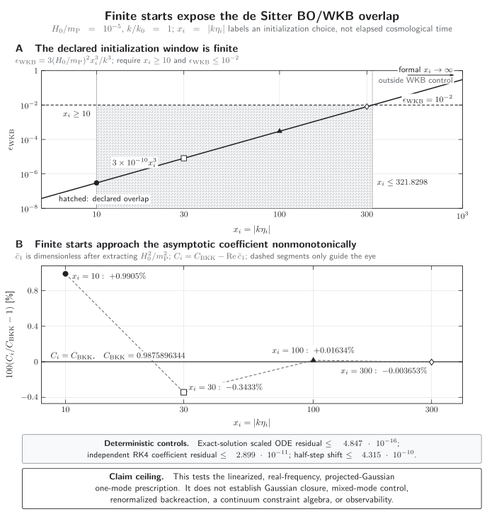
Finite-start control for the projected de Sitter one-mode benchmark. For $H_0/m_{\mathrm P}=10^{-5}$, $k/k_0=1$, $x_i=\lvert k\eta_i\rvert\ge10$, and $\epsilon_{\mathrm{WKB}}\le10^{-2}$, the declared initialization window is $10\le x_i\le321.8298$; the formal $x_i\to\infty$ state lies outside it. Starts at $x_i=10$, $30$, $100$, and $300$ approach $C_{\mathrm{BKK}}=0.9875896344$ nonmonotonically, with relative discrepancies $+0.9905\%$, $-0.3433\%$, $+0.01634\%$, and $-0.003653\%$. This tests the linearized real-frequency projected-Gaussian prescription, not Gaussian closure, mixed modes, renormalized backreaction, a continuum constraint algebra, or observability.

The plotted values and two independent numerical controls are reproduced below. The Runge–Kutta column compares direct evolution of the linearized Riccati equation with the exact incomplete-gamma solution; the half-step column changes the integration step and is an implementation check, not a physical error bar.

How to read this table. The first four columns reproduce the plotted starts and signed discrepancies. On narrow screens, swipe or focus the table and use Left/Right arrow keys; Home and End move to its edges.

Finite-start coefficients and deterministic integration controls

xi	εWKB	Ci	(Ci/CBKK − 1) × 100	|CiRK4 − Ci|	Half-step shift
10	3.0 × 10−7	0.997371864058125	+0.9905156308%	2.89895 × 10−11	4.31549 × 10−10
30	8.1 × 10−6	0.984199214150939	−0.3433025310%	2.84306 × 10−12	4.22826 × 10−11
100	3.0 × 10−4	0.987750987625295	+0.0163380880%	2.26430 × 10−12	3.59319 × 10−11
300	8.1 × 10−3	0.987553553773025	−0.0036533989%	2.29738 × 10−12	3.29921 × 10−11

Download the full-size SVG, numeric CSV, or semantic record. Across all four starts, the maximum exact-solution scaled ODE residual is $4.85\times10^{-16}$, the maximum independent-integration residual is $2.90\times10^{-11}$, and the maximum half-step shift is $4.32\times10^{-10}$.

This is a reproducible benchmark inside a declared projected prescription, not a universal prediction:

• a related canonical model has a solution ambiguity that permits enhancement or suppression Bini et al. 2013, §§ III–VII, especially Eqs. (6.4)–(6.7), pp. 8–10;
• slow-roll terms modify the coefficient at first slow-roll order Brizuela, Kiefer, and Krämer 2016b, Eqs. (88)–(89), p. 10;
• a clock-gauge-fixed inner product changes the perturbative measure and produces a late-time logarithm whose growth can invalidate fixed-order perturbation theory Chataignier and Krämer 2021, § IV.D, Eqs. (159)–(160), pp. 19–21;
• a Kuchař–Torre fluid clock with explicit graviton averaging gives a $k^{-3}$ suppression in its own de Sitter prescription Maniccia, Montani, and Tosoni 2024, Eq. (139), pp. 15–16; § VI.

This finite-mode benchmark establishes formal calculability and $m_{\mathrm P}^{-2}$ scaling within the declared split and projected state ansatz, after extrapolating the asymptotic state beyond the finite WKB overlap. It does not establish controlled evolution from $\eta=-\infty$. Its sign, coefficient, state shape, background response, and observational interpretation are not presently prescription independent.

What a controlled computation must record

How to read this table. Each row pairs a modelling choice with the check that can invalidate it. On narrow screens, swipe or focus the table and use Left/Right arrow keys to compare all four columns; Home and End move to its edges.

Inputs, primary controls, and failure signals at each layer of the calculation

Layer	Choice that must be stated	Primary control	Failure signal
Full functional theory	Spatial metric, matter fields, regulator, ordering, and operator domain	All local constraints, their algebra, and the physical inner product	Undefined products, an anomaly, or no continuum domain
Background	Variables, lapse, WKB branch, Hamilton principal function, and factor ordering	Hamilton–Jacobi and WKB transport residuals	A turning point or comparable amplitudes from neighboring branches
Physical mode	Gauge-invariant variable, Fourier normalization, state, and oscillator frequency	Linearized constraints, Wronskian, and normalizability	Gauge dependence or loss of normalizability
BO factorization	Slow/fast split, background-state basis, clock, inner product, and projected state family	Norm, off-diagonal background transitions, and background response at the retained order	The product state is not preserved or an observable changes outside the error budget
Background-state support	One WKB branch, a finite-width packet, or a coherent superposition	Repeat the observable across packet widths, phases, and trajectory prescriptions	Unbudgeted state- or trajectory-dependent spectral changes
Truncation	Box, mode set, cutoff, regulator, and renormalization prescription	Cutoff sequence, mixed-mode terms, and constraint-algebra residual	A false plateau, unsuppressed mixed terms, or a growing anomaly
Observable	Operator, evaluation time, pivot convention, and conversion to physical units	Independent Schrödinger- and Heisenberg-picture calculations	Fiducial-box, clock, or pivot dependence
Empirical claim	Transfer model, dataset, likelihood, nuisance parameters, and comparison baseline	Reproduce the baseline and vary the full analysis pipeline	The feature is degenerate, pipeline-dependent, or outside perturbative control

Useful dimensionless diagnostics include

$$\epsilon_{\mathrm{qg}}(k) =\left\lvert\frac{\delta\mathcal P(k)}{\mathcal P^{(0)}(k)}\right\rvert, \qquad \epsilon_{\mathrm{br}}(K) =\frac{ \left\lvert\sum_{k\le K} \langle\widehat{\mathcal H}_k\rangle_{\mathrm{ren}}\right\rvert} {m_{\mathrm P}^2\lvert V\rvert},$$

and, for an observable $O$ computed with cutoffs $K$ and $2K$,

$$\epsilon_{\mathrm{cut}}(K) =\frac{\lvert O_{2K}-O_K\rvert} {\max(\lvert O_{2K}\rvert,O_{\mathrm{floor}})}, \qquad \epsilon_{\mathrm{norm}} =\max_\eta \left\lvert\frac{\lVert\psi(\eta)\rVert^2} {\lVert\psi(\eta_i)\rVert^2}-1\right\rvert.$$

The expectation value in $\epsilon_{\mathrm{br}}$ must be renormalized; summing unrenormalized oscillator zero-point energies only measures the cutoff. The norm must use the declared physical inner product, not whichever auxiliary product is easiest to integrate. The positive $O_{\mathrm{floor}}$ prevents division by numerical noise when the reference observable is near zero; it must be declared, kept below the physically resolved scale, and varied to show that the conclusion is stable.

For the constraint algebra, the classical structure function contains the dynamical metric. A regulated construction must therefore publish the regulator, ordering, and common domain of the target operator, for example

$$\widehat{\mathcal B}_K[N,M] :=\operatorname{Ord}_K\!\left[ \int_\Sigma\mathrm d^3x\, \widehat h_K^{ab} (N\partial_bM-M\partial_bN) \widehat{\mathcal H}_{a,K} \right].$$

It can then monitor

$$\epsilon_{\mathrm{alg}}[N,M] =\frac{ \left\lVert \left([\widehat H_K[N],\widehat H_K[M]] -i\widehat{\mathcal B}_K[N,M]\right)\Psi_K \right\rVert} {\lVert\widehat H_K[N]\widehat H_K[M]\Psi_K\rVert +\lVert\widehat H_K[M]\widehat H_K[N]\Psi_K\rVert +\varepsilon_{\mathrm{floor}}}.$$

A small value for one pair of smearings is a unit test, not closure. The test set must probe different supports and gradients, and its tolerance must decrease along the continuum sequence. The positive $\varepsilon_{\mathrm{floor}}$ must be smaller than the resolved operator norms, and the result must be stable as it is lowered. If the construction claims a deformed rather than classical algebra, its declared target replaces $\widehat{\mathcal B}_K$. This diagnostic is unavailable in the reduced oscillator benchmark: the linearized constraints have already been solved, so no regulated representation of $\widehat H[N]$ and $\widehat D[\mathbf N]$ remains. It belongs to a separate functional, lattice, or mode construction that keeps those operators.

Adversarial test: add modes and change the split

A one-mode result can support more than a formal benchmark only if it survives attempts to break it.

1. Add the rest of the momentum shell and include $\sum_k\langle\widehat{\mathcal H}_k\rangle_{\mathrm{ren}}$ in the background Hamilton–Jacobi equation. Repeat until the observable and backreaction converge.
2. Double the ultraviolet cutoff at fixed physical volume, then enlarge the volume at fixed physical cutoff. These are different limits and must not be conflated.
3. Change the BO factorization or clock. Transform the inner product and conditional state consistently; compare relational observables, not raw wavefunctions.
4. In a separate regulated construction that retains the constraints, change factor ordering or regulator and evaluate $\epsilon_{\mathrm{alg}}$. Agreement of a power spectrum does not compensate for anomalous constraints.
5. Propagate both neighboring WKB branches. If their interference is comparable to the selected branch, stop using a single emergent time.

The mode-addition test already fails without further assumptions. For two commuting mode Hamiltonians,

$$\widehat H_{\mathrm{tot}}^2 =\widehat H_1^2+\widehat H_2^2 +2\widehat H_1\widehat H_2.$$

For two identical early-time oscillator vacua,

$$\langle\widehat H_i\rangle=\frac{k}{2}, \qquad \langle\widehat H_i^2\rangle=\frac{k^2}{4}.$$

The two retained self terms therefore sum to $k^2/2$, while the omitted mixed term also contributes $2\langle\widehat H_1\widehat H_2\rangle=k^2/2$. Product factorization supplies no suppression. Dropping such terms is a formal random-phase approximation whose regularization and range of validity must be demonstrated Chataignier and Krämer 2021, § IV.A, Eqs. (115)–(117).

Before the run, choose tolerances for $\epsilon_{\mathrm{qg}}$, $\epsilon_{\mathrm{br}}$, $\epsilon_{\mathrm{cut}}$, $\epsilon_{\mathrm{norm}}$, and, where available, $\epsilon_{\mathrm{alg}}$.

If every diagnostic is actually passed, the strongest conditional claim is: within a specified semiclassical branch, gauge-invariant mode truncation, clock, inner product, regulator, and convergence window, QFT on the background receives a calculable correction of order $m_{\mathrm P}^{-2}$.

The displayed one-mode benchmark tests sensitivity to one declared finite-time leading-correction matching rule inside the WKB window, but it does not establish a unique physically preferred finite-time state. It has not passed Gaussian-closure, mixed-mode, renormalized-backreaction, or continuum-algebra tests. Its present claim ceiling is the formal relative correction $O(\lambda_k)$ in the stated projected prescription.

Status through 30 August 2026

The one-mode calculation genuinely goes beyond a homogeneous wavefunction because $v_k$ carries spatial momentum and couples to the background variables. The benchmark does not solve a self-consistently corrected background equation. It also does not solve the full functional Wheeler–DeWitt equation, establish an anomaly-free continuum constraint algebra, or reconstruct general spacetime observables. Recent lattice work makes finite-dimensional metric positivity and lattice constraint corrections explicit, but the continuum physical theory remains a separate step.

Finite models now probe assumptions that the benchmark holds fixed. Exact evolution in a four-degree-of-freedom bouncing model does not generically preserve an initial background–perturbation product state; it produces entanglement and a small non-Gaussian component in the authors’ numerical fixture, which they explicitly present as a proof of concept rather than a generic prediction Bergeron, Małkiewicz, and Peter 2024, §§ II.D–III, Eqs. (17)–(20), pp. 4–5; § V, pp. 8–9. A perturbative extension derives a specific connected trispectrum, but its amplitude requires a model and its genericity and observability remain open Bergeron, Małkiewicz, and Peter 2025, § V.C, Eqs. (67)–(71), pp. 10–11; § VI, pp. 12–13.

Conversely, a 2026 construction retains BO factorization but allows a nonclassical superposition of background states. Its eikonal trajectories can change the tensor spectrum strongly and nonuniversally; the worked radiation-fluid bounce is deliberately incomplete and non-realistic, and generic scalar predictions and observational propagation are deferred Mazde, Mickel, and Peter 2026, §§ VII.B–VIII, pp. 12–16. These results are model evidence about factorization and background dependence, not detections of quantum gravity.

An unrefereed preprint submitted on 7 August 2026 examines a different source of state dependence: marginalizing the perturbation spectrum over a finite-width homogeneous Gaussian packet. In two simplified models with future de Sitter attractors, packet width modifies the spectrum and can generate corrections larger than the usual $m_{\mathrm P}^{-2}$ terms. The calculation neglects perturbative backreaction and nonadiabatic terms, omits $O(\hbar^2)$ contributions to the Mukhanov–Sasaki equation, and does not yet supply realistic potentials or generic observability Sonet, Tronconi, and Venturi 2026, § 4, Eqs. (52)–(54); § 5, Eqs. (67)–(74); § 6. It is evidence that background-state width matters, not a detection or a prescription-independent prediction.

No prescription-independent primordial signal has emerged from this program. For the BKK weak-coupling term, the scale $H_0^2/m_{\mathrm P}^2$ explains its tiny size, while the apparent $(k_0/k)^3$ growth warns where the fixed-order expansion fails rather than guaranteeing a large observable. The transferable initial-state output is a normalized finite-time kernel $\Omega_k(\eta_i)$ or density matrix, together with its clock, matching surface, pivot convention, and error budget—not the low-$k$ correction extrapolated outside its overlap window. That data is passed to Initial-State and Trans-Planckian Interfaces; branch selection, decoherence, and the claim ceiling continue on Semiclassical Recovery, Decoherence, Obstructions, and Status.

Common pitfalls

Calling one oscillator “full superspace.” A gauge-invariant mode is an honest inhomogeneous degree of freedom, but here it comes from a constraint-reduced quadratic action and mode coupling has been discarded. State the truncation before interpreting it.

Treating WKB time as fundamental. It is a derivative along one semiclassical branch, and this benchmark has already inserted conformal time into its oscillator frequency. At a turning point or during branch interference, the construction—not merely a numerical solver—has failed.

Forcing the corrected state to remain Gaussian. The Hamiltonian-squared term generates a quartic power of $v_k$. Projecting it away defines an approximation; it is not exact Gaussian evolution.

Quoting $0.988$ as a prediction of canonical quantum gravity. The number belongs to a particular background, BO split, projected Gaussian ansatz, initial condition, inner-product prescription, and reference-scale convention. The surviving lesson is the formal scaling and the need for an error budget.

Adding zero-point energy without renormalization. The raw sum over modes grows with the cutoff. A backreaction test must use the same renormalization prescription at every cutoff.

Checking only the naive norm. A nonconstant $L^2(\mathrm d v_k)$ norm may expose a bad effective Hamiltonian, or it may indicate that the auxiliary product is not the physical clock-conditioned product. Specify the measure before deciding which.

Exercises

Derive the Gaussian-width equation

Insert $\psi=N(\eta)e^{-\Omega(\eta)v^2/2}$ into

$$i\partial_\eta\psi =\frac12(-\partial_v^2+\omega^2v^2)\psi$$

and derive the equations for $N$ and $\Omega$.

Solution: derive the Gaussian-width equation

The derivatives are

$$\partial_v^2\psi=(\Omega^2v^2-\Omega)\psi, \qquad \partial_\eta\psi =\left(\frac{N'}N-\frac12\Omega'v^2\right)\psi.$$

Matching the $v^2$ coefficients gives

$$-\frac i2\Omega' =\frac12(-\Omega^2+\omega^2), \qquad i\Omega'=\Omega^2-\omega^2.$$

Matching the constant terms gives $iN'/N=\Omega/2$. Normalizability additionally requires $\operatorname{Re}\Omega>0$.

Recover freeze-out

Use

$$\Omega_k^{(0)} =\frac{k^3\eta^2}{1+k^2\eta^2} +\frac{i}{\eta(1+k^2\eta^2)}$$

to calculate $\langle v_k^2\rangle$ and the late-time limit of $\mathcal P_v(k)$.

Solution: recover freeze-out

For a normalized probability density proportional to $e^{-\operatorname{Re}\Omega\,v^2}$,

$$\langle v^2\rangle=\frac{1}{2\operatorname{Re}\Omega}.$$

Therefore

$$\mathcal P_v(k) =\frac{k^3}{4\pi^2} \frac{1+k^2\eta^2}{k^3\eta^2} =\frac{1+k^2\eta^2}{4\pi^2\eta^2}.$$

As $k\lvert\eta\rvert\to0$, $\mathcal P_v\to1/(4\pi^2\eta^2)$. The canonical variable grows as $a$, but $v/a$ approaches a constant; that is the physical freeze-out.

Locate the perturbative domain

For the benchmark correction

$$\delta_k=0.988\left(\frac{H_0}{m_{\mathrm P}}\right)^2 \left(\frac{k_0}{k}\right)^3,$$

find the condition on $k/k_0$ for $\delta_k<\delta_{\max}$. Evaluate it for $H_0/m_{\mathrm P}=10^{-5}$ and $\delta_{\max}=10^{-2}$.

Solution: locate the perturbative domain

Rearranging gives

$$\frac{k}{k_0} >\left[ \frac{0.988}{\delta_{\max}} \left(\frac{H_0}{m_{\mathrm P}}\right)^2 \right]^{1/3}.$$

For the stated values,

$$\frac{k}{k_0}>(9.88\times10^{-9})^{1/3} \approx2.15\times10^{-3}.$$

Below this scale, the formula’s growth announces loss of fixed-order control. It does not justify extrapolating the correction to arbitrarily small $k$.

Diagnose norm drift

Let the effective Hamiltonian be $\widehat H_{\mathrm eff}=\widehat H_R+i\widehat H_I$, where $\widehat H_R$ and $\widehat H_I$ are Hermitian in the chosen auxiliary product. Show how the norm changes.

Solution: diagnose norm drift

Using $i\lvert\psi'\rangle=\widehat H_{\mathrm eff}\lvert\psi\rangle$,

$$\frac{\mathrm d}{\mathrm d\eta}\langle\psi\vert\psi\rangle =i\langle\psi\vert (\widehat H_{\mathrm eff}^{\dagger}-\widehat H_{\mathrm eff}) \vert\psi\rangle =2\langle\widehat H_I\rangle.$$

Thus the auxiliary norm is conserved only if $\langle\widehat H_I\rangle=0$ for the relevant states. A consistent BO treatment may instead shift the corresponding term into backreaction or the physical inner-product measure; either move must be stated and checked.

Count the mixed-mode terms

For $N$ identical independent oscillator vacua with

$$\widehat H_{\mathrm{tot}}=\sum_{i=1}^N\widehat H_i, \qquad \widehat H_i\lvert0\rangle=\frac{k}{2}\lvert0\rangle,$$

compare the self terms and mixed terms in $\langle\widehat H_{\mathrm{tot}}^2\rangle$. At what $N$ are the mixed terms parametrically negligible?

Solution: count the mixed-mode terms

Expanding the square gives

$$\widehat H_{\mathrm{tot}}^2 =\sum_{i=1}^N\widehat H_i^2 +\sum_{i\ne j}\widehat H_i\widehat H_j.$$

There are $N$ self terms and $N(N-1)$ ordered mixed terms. Product factorization gives

$$\left\langle\sum_i\widehat H_i^2\right\rangle =\frac{Nk^2}{4}, \qquad \left\langle\sum_{i\ne j}\widehat H_i\widehat H_j\right\rangle =\frac{N(N-1)k^2}{4}.$$

The mixed-to-self ratio is $N-1$. It is already unity for two modes and grows with the mode count, so independence of the state does not suppress the cross terms. A separate approximation, regulator, and convergence test would be needed to discard them.

For a compact chapter-level orientation, use the structure diagram and validity and failure diagram. The claim-domain table compares assumptions, counterevidence, falsifiers, and conclusions across the chapter.

References

• Bergeron, H., P. Małkiewicz, and P. Peter. “Quantum Entanglement and Non-Gaussianity in the Primordial Universe.” Physical Review D 110 (2024): 043512. DOI. Open PDF.
• Bergeron, H., P. Małkiewicz, and P. Peter. “Non-Gaussianities as a Signature of Quantumness of Quantum Cosmology.” Physical Review D 112 (2025): 063558. DOI. Open PDF.
• Bini, D., G. Esposito, C. Kiefer, M. Krämer, and F. Pessina. “On the Modification of the Cosmic Microwave Background Anisotropy Spectrum from Canonical Quantum Gravity.” Physical Review D 87 (2013): 104008. DOI. Open PDF.
• Brizuela, D., C. Kiefer, and M. Krämer. “Quantum-Gravitational Effects on Gauge-Invariant Scalar and Tensor Perturbations during Inflation: The de Sitter Case.” Physical Review D 93 (2016a): 104035. DOI. Open PDF.
• Brizuela, D., C. Kiefer, and M. Krämer. “Quantum-Gravitational Effects on Gauge-Invariant Scalar and Tensor Perturbations during Inflation: The Slow-Roll Approximation.” Physical Review D 94 (2016b): 123527. DOI. Open PDF.
• Chataignier, L., C. Kiefer, and P. Moniz. “Observations in Quantum Cosmology.” Classical and Quantum Gravity 40 (2023): 223001. DOI. Open PDF.
• Chataignier, L., and M. Krämer. “Unitarity of Quantum-Gravitational Corrections to Primordial Fluctuations in the Born–Oppenheimer Approach.” Physical Review D 103 (2021): 066005. DOI. Open PDF.
• Friedman, J. L., and I. Jack. “Formal Commutators of the Gravitational Constraints Are Not Well Defined: A Translation of Ashtekar’s Ordering to the Schrödinger Representation.” Physical Review D 37 (1988): 3495–3504. DOI.
• Halliwell, J. J., and S. W. Hawking. “Origin of Structure in the Universe.” Physical Review D 31 (1985): 1777–1791. DOI.
• Kiefer, C., and T. P. Singh. “Quantum Gravitational Corrections to the Functional Schrödinger Equation.” Physical Review D 44 (1991): 1067–1076. DOI.
• Kiefer, C., and D. Wichmann. “Semiclassical Approximation of the Wheeler–DeWitt Equation: Arbitrary Orders and the Question of Unitarity.” General Relativity and Gravitation 50 (2018): 66. DOI. Open PDF.
• Lang, T., and S. Schander. “Quantum Geometrodynamics Revived I: Classical Constraint Algebra.” Classical and Quantum Gravity 41 (2024a): 185004. DOI. Open PDF.
• Lang, T., and S. Schander. “Quantum Geometrodynamics Revived II: Hilbert Space of Positive Definite Metrics.” Classical and Quantum Gravity 41 (2024b): 185003. DOI. Open PDF.
• Maniccia, G., G. Montani, and M. Tosoni. “Analyzing the Influence of Graviton Fluctuations on the Inflationary Spectrum with a Kuchař–Torre Clock.” Physical Review D 110 (2024): 086012. DOI. Open PDF.
• Mazde, K., L. Mickel, and P. Peter. “Quantum Cosmological Background Superposition and Perturbation Predictions.” Physical Review D 113 (2026): 026011. DOI. Open PDF.
• Sonet, S., A. Tronconi, and G. Venturi. “Quantum-Cosmological Corrections to Inflationary Spectra from Gaussian Wave Packets.” arXiv:2608.07164v1 [gr-qc] (7 August 2026). arXiv. Open PDF.
• Teitelboim, C. “How Commutators of Constraints Reflect the Spacetime Structure.” Annals of Physics 79 (1973): 542–557. DOI.