Replica Wormholes and Saddle Competition

A replica wormhole is one possible bulk filling of a replicated gravitational boundary problem; it is not the cyclic boundary sewing itself. In the microcanonical Jackiw–Teitelboim (JT) gravity model with an end-of-the-world brane, the second moment of a $k$-state reference system receives a disconnected contribution $1/k$ and a connected contribution $1/d_B$, where $d_B$ is the effective number of black-hole states in the chosen energy window. Their magnitudes cross at $k=d_B$. The full answer is a sum, however: partial replica connectivities become leading near the crossover for $n\geq3$, and a controlled integer-$n$ crossing does not by itself determine the $n\to1$ entropy.

Required background. Semiclassical Gravitational Replicas defines the integer-$n$ boundary problem and its normalized moment. Fixed-Theory, Ensemble, and Superselection Claims supplies the interpretation boundary used below.

Helpful background. JT Topological Expansion and Weil–Petersson Volumes explains the topology expansion. Quantum Extremal Surfaces: Renormalized Semiclassical Definition owns the renormalized generalized-entropy functional that appears only after a valid continuation.

Replica topology becomes a saddle label

For a normalized density matrix $\rho_R$, the exact replica observables are

$$P_n(R)=\operatorname{Tr}\rho_R^n =\frac{Z_n[R]}{Z_1^n}, \qquad S_n(R)=\frac{\log P_n(R)}{1-n}, \qquad P_1(R)=1.$$

At an integer $n\geq2$, first fix the state preparation, the cyclic sewing on $R$, all nongravitating boundary conditions, and the gravitational integration domain. Several fillings of those same data may then contribute. Before selecting any dominant one-copy saddle, the normalized semiclassical expression is

$$P_n(\lambda)\simeq \frac{ \displaystyle\sum_{a\in\mathcal A_n} m_{n,a}\nu_{n,a}\mathcal D_{n,a}(\lambda) e^{-I^{\mathrm{ren}}_{n,a}(\lambda)} }{ \displaystyle\left[ \sum_{b\in\mathcal A_1} m_{1,b}\nu_{1,b}\mathcal D_{1,b}(\lambda) e^{-I^{\mathrm{ren}}_{1,b}(\lambda)} \right]^n }.$$

Here $\mathcal D$ is the gauge-fixed determinant and moduli factor, $\nu$ is the contour or thimble coefficient, and $m$ is an orbit or combinatorial multiplicity. Keeping $\nu$ and $m$ separate matters: contour membership can change while the number of symmetry-related fillings does not. The labels include topology, replica permutation, and any symmetry-breaking pattern.

Only if a single one-copy saddle $0$ controls the denominator may its contribution be factored out and the compact form

$$P_n(\lambda)\simeq \sum_{a\in\mathcal A_n} c^{\mathrm{rel}}_{n,a}\widehat{\mathcal D}_{n,a}(\lambda) e^{-\mathcal I^{\mathrm{cl}}_{n,a}(\lambda)} \left[1+O(g_{\mathrm{sc}})\right]$$

be used, with

$$c^{\mathrm{rel}}_{n,a} \equiv \frac{m_{n,a}\nu_{n,a}}{(m_{1,0}\nu_{1,0})^n}, \qquad \mathcal I^{\mathrm{cl}}_{n,a} =I^{\mathrm{ren}}_{n,a}-nI^{\mathrm{ren}}_{1,0}, \qquad \widehat{\mathcal D}_{n,a} =\frac{\mathcal D_{n,a}}{\mathcal D_{1,0}^{\,n}}.$$

Thus the compact coefficient is explicitly relative to the controlling one-copy saddle; choosing $m_{1,0}\nu_{1,0}=1$ is only a normalization convention. The declared correction $g_{\mathrm{sc}}$ includes the subleading one-copy saddles as well as the stated loop and topology corrections.

For positive, noninterfering terms it is convenient to absorb their magnitudes into an effective exponent,

$$\Gamma_{n,a} =\operatorname{Re}\mathcal I^{\mathrm{cl}}_{n,a} -\log\left\lvert c^{\mathrm{rel}}_{n,a}\widehat{\mathcal D}_{n,a}\right\rvert .$$

Two contributions have equal magnitude where $\Gamma_{n,a}=\Gamma_{n,b}$. This is often called an anti-Stokes condition. A Stokes locus instead concerns alignment of phases and a possible change of thimble coefficients. Thus “the smaller action wins” is licensed only when both coefficients are nonzero on the declared contour, the same counterterms and normalization were used, phases do not cancel decisively, fluctuation operators are treated consistently, and no omitted saddle is larger.

Here disconnected means that the dynamical-gravity filling has separate replica components. The nongravitating boundary sheets used to take the trace are still cyclically sewn. A replica wormhole is a filling whose dynamical-gravity region connects replicas. Neither option is a Lorentzian signal channel.

The microcanonical JT–brane laboratory

The Penington–Shenker–Stanford–Yang model supplies a compact calculation in which topology and index counting can both be followed. JT gravity contains an end-of-the-world (EOW) brane with $k$ orthogonal labels, entangled with a nongravitating reference $R$. The path-integral preparation is written schematically as

$$\lvert\widetilde\Psi\rangle =\frac{1}{\sqrt{k}} \sum_{i=1}^{k} \lvert\psi_i\rangle_B\lvert i\rangle_R .$$

In the dimensionless normalization of the source, the Euclidean action and its two kinds of boundary data are

$$\begin{aligned} I&=I_{\mathrm{JT}}+\mu\int_{\mathrm{EOW}}d\ell, \\ I_{\mathrm{JT}} &=-\frac{S_0}{2\pi}\left[ \frac12\int_{\mathcal M}\!\sqrt g\,\mathcal R +\int_{\partial\mathcal M}\!\sqrt h\,K \right] \\ &\quad-\left[ \frac12\int_{\mathcal M}\!\sqrt g\,\phi(\mathcal R+2) +\int_{\partial\mathcal M}\!\sqrt h\,\phi K \right], \end{aligned}$$ $$\left.ds^2\right|_{\partial\mathcal M} =\frac{d\tau^2}{\epsilon^2}, \qquad \left.\phi\right|_{\partial\mathcal M}=\frac1\epsilon, \qquad \epsilon\to0,$$ $$\left.K\right|_{\mathrm{EOW}}=0, \qquad \left.\partial_n\phi\right|_{\mathrm{EOW}}=\mu, \qquad \mu\geq0.$$

Here $\mathcal R$ is the two-dimensional scalar curvature, $K$ is the extrinsic curvature, and $\mu$ is the EOW-brane mass. These equations fix what “the JT–brane model” means below; they are Penington et al. 2022, § 2.1, eqs. (2.1)–(2.4).

For one ensemble member, let $G_{ij}=\langle\psi_j\vert\psi_i\rangle$. The exact reduced density matrix and the mean-normalized matrix used in the leading gravity expansion are different:

$$\rho_R=\frac{G}{\operatorname{Tr}G}, \qquad \widehat\rho_R=\frac{G}{kZ_1}, \qquad Z_1\equiv\mathbb E G_{ii}.$$

Thus $\operatorname{Tr}\rho_R=1$ in every member, while only $\mathbb E\operatorname{Tr}\widehat\rho_R=1$. The difference is a normalization fluctuation that is subleading in the planar regime but must not be hidden when an exact finite-dimensional statement is made. To keep the two observables distinct, write

$$\widehat P_n^{\mathrm{planar}} \equiv \left[ \mathbb E\operatorname{Tr}\widehat\rho_R^n \right]_{\mathrm{leading\ planar}}.$$

$P_n$ without a hat continues to mean the exact, sample-normalized moment of $\rho_R$.

The model declaration is:

Entry	Declaration
Gravity sector	Euclidean JT gravity with an EOW-brane boundary condition and the stated topology sum
State	The path-integral preparation above, with samplewise normalization $\rho_R=G/\operatorname{Tr}G$; $R$ is nongravitating and $B$ is the black-hole system
Observable	Exact $P_n=\operatorname{Tr}\rho_R^n$; the leading gravity calculation first evaluates ensemble moments of $\widehat\rho_R=G/(kZ_1)$ at positive integer $n$
Control parameter	$k$, the reference dimension, compared with the effective microcanonical dimension $d_B$
Energy prescription	A narrow window of width $\Delta s$ about $s_\star$, held fixed across replicas
Approximation	Leading planar topology sum at large $k$ and $d_B$, with handle, window, determinant, and normalization corrections stated separately
Logical status	An ensemble-completed solvable gravity model, not a theorem about a generic fixed boundary theory

The model’s matrix-integral/ensemble completion supplies the topology weights retained in this calculation. It is not an independently established Lefschetz-thimble decomposition of a unique Euclidean metric contour. The generic contour interventions used later are therefore stress tests of the inference, not alternate contours computed inside this fixture.

Let $Z_m$ denote the disk amplitude with $m$ alternating asymptotic-boundary and EOW-brane segments. The two $n=2$ fillings have different numbers of brane-label loops. Including the normalization $(kZ_1)^2$ gives

$$\begin{aligned} \mathbb E\operatorname{Tr}\widehat\rho_R^2 &=\frac{kZ_1^2+k^2Z_2}{(kZ_1)^2} \\ &=\underbrace{\frac1k}_{\text{disconnected gravity filling}} +\underbrace{\frac{Z_2}{Z_1^2}}_{\text{connected replica wormhole}} . \end{aligned}$$

The first numerator has one $k$-index loop and two gravitational disks; the second has two index loops and one connected filling. This leading planar formula neglects the difference between $kZ_1$ and the fluctuating $\operatorname{Tr}G$. The finite-dimensional check below isolates the size of that effect using a separately sample-normalized Haar ensemble; it does not retroactively make $\widehat\rho_R$ samplewise normalized. The gravity derivation and its ensemble dual are developed in Penington et al. 2022, §§ 2.1–2.5 and Appendix D.

For this action, the spectral density without the topological factor and the weight of one alternating asymptotic/EOW segment are

$$\rho_0(s)=\frac{s}{2\pi^2}\sinh(2\pi s), \qquad \boldsymbol\rho(s)=e^{S_0}\rho_0(s),$$ $$y(s)=e^{-\beta s^2/2}\, 2^{1-2\mu} \left\lvert \Gamma\!\left(\mu-\frac12+is\right) \right\rvert^2.$$

Thus $\beta$ is the renormalized asymptotic-boundary length, while $\mu$ controls the EOW-brane weight. These functions follow from Penington et al. 2022, § 2.5, eqs. (2.30)–(2.34). Let the microcanonical window be

$$W=\left[s_\star-\frac{\Delta s}{2},s_\star+\frac{\Delta s}{2}\right],$$

and define its effective dimension and replicated disk amplitudes exactly by

$$d_B=e^{\mathbf S} =\int_W ds\,\boldsymbol\rho(s), \qquad Z_n(W)=\int_W ds\,\boldsymbol\rho(s)y(s)^n.$$

Here $y(s)>0$ is the state-preparation and EOW-brane weight contributed by each asymptotic segment. If it varies negligibly across $W$, then

$$q_n\equiv\frac{Z_n(W)}{Z_1(W)^n} =d_B^{1-n}\left[1+O(\epsilon_{\mathrm{win}})\right], \qquad d_B\simeq\boldsymbol\rho(s_\star)\Delta s.$$

The exact integral definition absorbs variation of the density of states; the narrow-window error below controls the remaining variation of $y(s)$. The bold density includes the JT topological factor and the energy-dependent density of states. Therefore $d_B$ must not be silently replaced by $e^{S_0}$: $S_0$ controls topology, whereas $\mathbf S=\log d_B$ is the entropy of the chosen microcanonical window. The purity becomes

$$\widehat P_2^{\mathrm{planar}} =\frac1k+\frac1{d_B},$$

so the endpoint effective exponents and their difference are

$$\Gamma_{2,\mathrm{disc}}=\log k, \qquad \Gamma_{2,\mathrm{wh}}=\log d_B, \qquad \Delta\Gamma_2=\log\frac{d_B}{k}.$$

The magnitudes cross at

$$\boxed{k_\star=d_B} \qquad\Longleftrightarrow\qquad \log k_\star=\mathbf S .$$

Before making the sharp-window approximation, retain the exact $q_2=Z_2(W)/Z_1(W)^2$. The actual leading crossing is $k_\star=q_2^{-1}$ when both terms are positive and admitted. A changed brane condition or energy prescription changes $q_2$ and therefore moves or can remove the crossing; a genuine bath coupling can also change the observable and the admitted saddle families.

One numerical fixture makes every scale checkable. In the source normalization, choose

$$\mu=1,\qquad \beta=0.2,\qquad s_\star=1,\qquad \Delta s=10^{-3}, \qquad S_0=8.459208506794.$$

The quoted $S_0$ is chosen so that this window has $d_B=64$. Direct quadrature then gives

$$\int_W\rho_0(s)\,ds=0.0135641442035, \qquad d_B=64,$$ $$q_2=0.0156250144376, \qquad k_\star=q_2^{-1}=63.9999408635.$$

The sharp-window crossing is therefore shifted by only $9.24\times10^{-7}$ in relative terms. At $k=64$, $\Gamma_{2,\mathrm{disc}}=\log64=4.15888308336$ while $-\log q_2=4.15888215935$. This small location shift should not be confused with the much larger failure of an endpoint-only approximation at the crossover.

The full crossover, not just two endpoints

Planar replica connectivities

For $n\geq3$, “fully disconnected” and “fully connected” are only the two endpoints of a larger sum. In the microcanonical planar regime, the moment is

$$\widehat P_n^{\mathrm{planar}} =k^{1-n} \sum_{j=1}^{n} N(n,j)\left(\frac{k}{d_B}\right)^{j-1}, \qquad N(n,j)=\frac1n\binom nj\binom n{j-1},$$

where the Narayana number $N(n,j)$ counts noncrossing replica permutations with the required cycle count. In the notation of Penington et al., their subsystem dimensions $k$ and $e^{\mathbf S}$ are $k$ and $d_B$ here; the permutation and Narayana formulas are Penington et al. 2022, Appendix E, eqs. (E.1)–(E.4). Moment fluctuations are suppressed in the stated large-dimension planar regime. The endpoint terms are $k^{1-n}$ and $d_B^{1-n}$, but the intermediate connectivities are not small near $k=d_B$. For example,

$$\widehat P_3^{\mathrm{planar}} =\frac1{k^2}+\frac{3}{k d_B}+\frac1{d_B^2}.$$

At the crossing, the three orbit-summed classes occur in the ratio $1:3:1$. Each individual transposition has the same weight as either endpoint there; the partial class is larger because it contains three noncrossing transpositions. A two-endpoint minimum is therefore least reliable exactly where the endpoint effective exponents meet. More generally, the sum of the Narayana numbers is the Catalan number $C_n$, and at $k=d_B$

$$\widehat P_n^{\mathrm{planar}}=C_n k^{1-n}, \qquad \widehat S_{n,\mathrm{ann}}^{\mathrm{planar}} =\log k-\frac{\log C_n}{n-1}.$$

Here $\widehat S_{n,\mathrm{ann}}^{\mathrm{planar}}\equiv\log\widehat P_n^{\mathrm{planar}}/(1-n)$ is annealed with respect to the gravity ensemble. This is the uniform planar description of the crossover, rather than “determinant smoothing” of two isolated terms.

Exact finite-dimensional checkpoint

There is a useful independent normalization check. Let $\lvert\Psi\rangle$ be Haar-random in $\mathbb C^k\otimes\mathbb C^{d_B}$, now taking $d_B$ to be an integer. With $D=kd_B$ and $F_R$ the swap on two copies of $R$,

$$\operatorname{Tr}\rho_R^2 =\operatorname{Tr}\!\left[ \lvert\Psi\rangle\!\langle\Psi\rvert^{\otimes2} (F_R\otimes\mathbf1_{BB}) \right].$$

The Haar second moment is

$$\mathbb E\!\left[ \lvert\Psi\rangle\!\langle\Psi\rvert^{\otimes2} \right] =\frac{\mathbf1+F_R\otimes F_B}{D(D+1)}.$$

Taking the traces gives $\operatorname{Tr}F_R=k$, $\operatorname{Tr}F_B=d_B$, and hence

$$\mathbb E P_2 =\frac{k d_B^2+k^2d_B}{kd_B(kd_B+1)} =\frac{k+d_B}{kd_B+1}.$$

The two algebraic contractions can be written

$$P_{2,\mathrm{id}}^{\mathrm{Haar}} =\frac{d_B}{kd_B+1}, \qquad P_{2,\mathrm{swap}}^{\mathrm{Haar}} =\frac{k}{kd_B+1}.$$

The identity and swap contractions approach $1/k$ and $1/d_B$ at large dimensions, their ratio is exactly $k/d_B$, and they cross at $k=d_B$. Haar integration carries no intrinsic bulk topology: only their large-dimension weights match the disconnected and replica-wormhole endpoint scalings of the PSSY model. This is a finite-dimensional random-state checkpoint, not an assertion that a Haar state is the exact microscopic dual of every gravitational model. The same purity formula appears in Życzkowski and Sommers 2001, eq. (44) and the early random-subsystem analysis of Lubkin 1978, pp. 1028–1031.

Taking the logarithm after the ensemble average defines the annealed second Rényi quantity

$$S_{2,\mathrm{ann}}^{\mathrm{Haar}} \equiv-\log\mathbb E P_2 =\log(kd_B+1)-\log(k+d_B).$$

It is not the quenched average $\mathbb E S_2=\mathbb E[-\log P_2]$: expectation and logarithm do not commute, and Jensen’s inequality gives $\mathbb E S_2>S_{2,\mathrm{ann}}^{\mathrm{Haar}}$ whenever the purity fluctuates. This annealed quantity is the appropriate finite-dimensional comparison for a gravitational calculation that averages the replicated moment before taking its logarithm; the distinction is emphasized in de Boer, Hollander, and Rolph 2024, § 1, eqs. (1.5)–(1.6).

Let $m=\min(k,d_B)$ and $M=\max(k,d_B)$. The dominant-contraction estimate is $S_2^{\mathrm{dom}}=\log m$, and its exact error is

$$\begin{aligned} \delta_{2,\mathrm{ann}} &=S_2^{\mathrm{dom}}-S_{2,\mathrm{ann}}^{\mathrm{Haar}} \\ &=\log\!\left(1+\frac mM\right) -\log\!\left(1+\frac1{mM}\right), \\ 0\leq\delta_{2,\mathrm{ann}} &\leq\log\!\left(1+\frac mM\right) \leq\frac mM . \end{aligned}$$

Thus the endpoint approximation is parametrically accurate far from the crossover. At $k=d_B=d$ it misses

$$\delta_{2,\mathrm{ann}}=\log2-\log(1+d^{-2}),$$

which approaches $\log2$, not zero, as the dimensions grow. The figure puts the planar connectivity sum and this finite normalization check side by side.

On a narrow screen, swipe or use the Left and Right arrow keys to pan across the figure. Home and End move to its edges. A full-size link is also available.

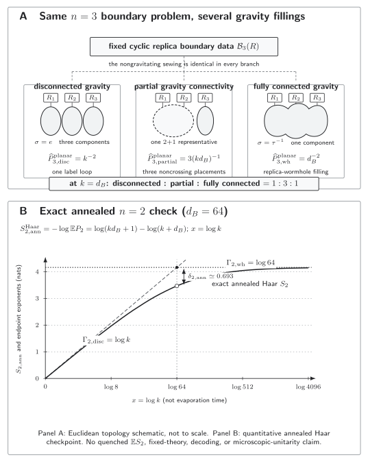
The same $n=3$ cyclic boundary data admit disconnected, partially connected, and fully connected dynamical-gravity fillings. In the microcanonical planar model their contributions at $k=d_B$ occur in the ratio $1:3:1$, so the intermediate class cannot be discarded near the endpoint crossing. The lower panel fixes $d_B=64$ and compares $S_{2,\mathrm{ann}}^{\mathrm{Haar}}=-\log\mathbb E P_2$ with the endpoint exponents $\log k$ and $\log d_B$; the exact annealed sum lies below their lower envelope by almost $\log2$ at $k=d_B$. It does not plot the quenched average $\mathbb E S_2$. The horizontal axis is $\log k$, not time. Euclidean topology schematic and quantitative finite-dimensional checkpoint; no microscopic-unitarity or fixed-theory claim. Accessible figure data (JSON)

The figure has the following text-equivalent content.

Displayed element	Exact relation	Approximation or condition	What it does not imply
Common top banner	One fixed cyclic boundary problem $\mathcal B_3(R)$	Integer $n=3$	That sewing selects a bulk topology
Disconnected class	Contribution $k^{-2}$	Planar microcanonical PSSY model	A disconnected nongravitating trace
Partial class	Total contribution $3/(kd_B)$	Three noncrossing transpositions	A negligible correction at the crossing
Fully connected class	Contribution $d_B^{-2}$	Admitted replica-wormhole topology	A Lorentzian bridge or signal path
Lower plot	$S_{2,\mathrm{ann}}=-\log\mathbb E P_2=\log(kd_B+1)-\log(k+d_B)$	Haar state with $d_B=64$	The quenched average $\mathbb E S_2$ or exact finite-$G_N$ gravity
Crossing gap	$\log2-\log(1+d_B^{-2})$	$k=d_B$ in the annealed quantity	A sharp exact phase transition

A reproducible error budget

The crossing is meaningful only relative to declared remainders. Five distinct controls should not be collapsed into one ellipsis.

1. Planar versus nonplanar terms. In the JT genus expansion, each added handle is typically suppressed by $e^{-2S_0}$. Finite-dimensional contraction nonplanarity is a separate expansion. For example, the exact Haar third moment is

   $$\mathbb E P_3 =\frac{k^2+3kd_B+d_B^2+1} {(kd_B+1)(kd_B+2)}.$$

   The first three numerator terms are the planar $1:3:1$ classes after large-dimension normalization; the final $+1$ is the crossed permutation. At $k=d_B=d$, it is down by $d^{-2}$ relative to either planar endpoint. Near the crossing, use the complete planar permutation sum before estimating either crossed contractions or JT handles.

2. Energy-window error. With the exact window integrals defined above, a conservative logarithmic bound is

   $$\epsilon_{\mathrm{win}} \equiv \left\lvert\log\!\left(q_nd_B^{n-1}\right)\right\rvert \lesssim n\,\Delta s \sup_{s\,\mathrm{in\ window}} \left\lvert\partial_s\log y(s)\right\rvert .$$

   The microcanonical reduction requires this quantity to be small and $d_B\gg1$. Because $d_B$ is the integrated density, no separate freezing of $\boldsymbol\rho(s)$ is hidden in this estimate.

3. Normalization and finite dimension. The planar purity omits state-normalization fluctuations. The exact Haar expression shows their scale explicitly through $1/(kd_B)$ and remains normalized even when one dimension is small.

4. Prefactors and contour coefficients. If the positive endpoint terms are $C_d/k$ and $C_w/d_B$, then

   $$\log k_\star =\log d_B+\log\frac{C_d}{C_w}.$$

   A vanishing $C_w$, a negative mode requiring a different contour treatment, or destructive phase interference can erase the simple crossing rather than merely shift it.

5. Crossing-location uncertainty. For a general control $\lambda$, let $\Delta\Gamma_n(\lambda)=\Gamma_{n,\mathrm{wh}}-\Gamma_{n,\mathrm{disc}}$. A perturbation shifts a simple crossing by

   $$\delta\lambda_\star =-\frac{\delta\Delta\Gamma_n(\lambda_\star)} {\partial_\lambda\Delta\Gamma_n(\lambda_\star)}.$$

   If $\lvert\delta\Delta\Gamma_n\rvert\leq\epsilon_\Gamma$ bounds the error in the effective-exponent difference, endpoint dominance is robust only where $\lvert\Delta\Gamma_n\rvert>\epsilon_\Gamma$. Inside that band, the honest result is “crossover unresolved at this order.”

For the numerical fixture above at $n=2$ and $k=64$, the scales separate as follows:

Effect	Reproducible value or bound
Conservative window bound	$\epsilon_{\mathrm{win}}\leq6.66\times10^{-3}$
Direct relative shift of $k_\star$	$9.24\times10^{-7}$
One-handle scale	$e^{-2S_0}=4.49\times10^{-8}$
Haar normalization and crossed-contraction scales	$1/(kd_B)=2.44\times10^{-4}$
Error of the endpoint-only annealed Haar estimate at the crossing	$0.69290307$

The first line follows by inserting $\mu=1$ into $y(s)$, for which $\partial_s\log y=-\beta s-\pi\tanh(\pi s)$, and taking the supremum over $W$. The endpoint omission is therefore the dominant demonstrated error at the crossover: the full planar sum is compulsory there. These checks are reproducible because each changes an explicit input or retained class. They also show why a plotted cusp in a leading minimum is not an uncertainty estimate.

Why integer dominance does not determine the entropy

For a finite Haar-random bipartite state, all moments have the exact permutation formula

$$\mathbb E P_n =\frac{1}{(kd_B)_n} \sum_{\sigma\in S_n} k^{C(\tau\sigma)}d_B^{C(\sigma)}, \qquad \tau=(1\,2\,\ldots n),$$

where $(D)_n=D(D+1)\cdots(D+n-1)$ and $C(\sigma)$ counts cycles. The identity permutation produces the disconnected endpoint; $\tau^{-1}$ produces the fully connected endpoint; the remaining permutations supply partial and nonplanar terms. Keeping only permutations that maximize $C(\sigma)+C(\tau\sigma)=n+1$ gives the planar Narayana sum. The exact permutation formula and this reduction are Penington et al. 2022, Appendix E, eqs. (E.1)–(E.4), after relabeling their two subsystem dimensions as $k$ and $d_B$.

For an actual finite density matrix, $P(z)=\sum_i\lambda_i^z$ is defined for $\operatorname{Re}z>0$, so its continuation is fixed by the spectrum. A gravitational calculation generally supplies only selected integer moments and their saddle decompositions. Those data do not automatically provide the spectrum or a unique term-by-term continuation.

The exact von Neumann entropy is

$$S(R)=-\left.\partial_n\log P_n(R)\right|_{n=1}.$$

In the microcanonical PSSY model, an extra continuation principle is actually available: the complete planar topology sum obeys a Schwinger–Dyson equation. With

$$R(\lambda)=\operatorname{Tr}\frac1{\lambda-\widehat\rho_R},$$

the sharp-window equation and its spectral density are

$$R(\lambda)^2+ \left(\frac{d_B-k}{\lambda}-kd_B\right)R(\lambda) +\frac{k^2d_B}{\lambda}=0,$$ $$\begin{aligned} D(\lambda) &=\frac{kd_B}{2\pi\lambda} \sqrt{(\lambda-\lambda_-)(\lambda_+-\lambda)} +(k-d_B)_+\,\delta(\lambda), \\ \lambda_\pm &=\left(k^{-1/2}\pm d_B^{-1/2}\right)^2 . \end{aligned}$$

The continuous term is supported on $\lambda_-\leq\lambda\leq\lambda_+$. This is the Page, or Marchenko–Pastur, spectrum, including the zero-eigenvalue multiplicity when $k>d_B$. It fixes the planar continuation and gives, for $m=\min(k,d_B)$ and $M=\max(k,d_B)$,

$$S_{\mathrm{planar}}(R) =-\int d\lambda\,D(\lambda)\lambda\log\lambda =\log m-\frac{m}{2M} +O\!\left(\frac1{mM}\right).$$

The resolvent, density, and entropy integral are Penington et al. 2022, § 2.5.1, eqs. (2.35)–(2.38). Separately, exact finite-dimensional Haar integration gives

$$\mathbb E S(R) =H_{mM}-H_M-\frac{m-1}{2M} =\log m-\frac{m}{2M}+O\!\left(\frac1{mM}\right).$$

Here $H_r=\sum_{j=1}^rj^{-1}$. Page 1993, pp. 1291–1294 conjectured this finite formula, and Sen 1996, pp. 1–3 proved it. It is a quenched von Neumann average obtained from the full spectrum, not by differentiating the single annealed $n=2$ checkpoint. At $k=d_B=d$, for example, it approaches $\log d-1/2$, whereas $S_{2,\mathrm{ann}}$ approaches $\log d-\log2$. The distinction is physical Rényi-index dependence, not an error bar.

A single branch may yield

$$S_a =\left.\partial_n\Gamma_{n,a}\right|_{n=1}$$

only if it belongs to a controlled family reaching the physical $n=1$ geometry, has the correct normalization there, and controls a punctured neighborhood of $n=1$. Naively continuing two unit-prefactor endpoint terms would give $P_1=2$, exposing the mistake: the saddle descriptions can coalesce, reorganize, or require a uniform sum at one.

The finite-$n$ equation $\Delta\Gamma_n(\lambda_n^\star)=0$ is therefore distinct from equality of candidate endpoint entropies,

$$\left.\partial_n\Gamma_{n,a}\right|_{n=1} = \left.\partial_n\Gamma_{n,b}\right|_{n=1}.$$

Even this latter comparison is meaningful only when both smooth, correctly normalized, noninterfering families reach the same physical $n=1$ geometry. The finite-dimensional full entropy is smooth, so equality of endpoint estimates is not generically a literal phase transition. Replica symmetry must also be checked rather than inferred; a symmetry-breaking saddle has an orbit of images and does not admit the usual one-fundamental-domain quotient.

Evidence status, checked 30 August 2026. Explicit JT calculations continue to support replica-wormhole contributions in controlled models, including finite-$n$ backreaction analyses Hollowood, Kumar, and Piper 2024, §§ 3, 5, and 7–8 and real-time wavefunction constructions reproducing Euclidean or complex Rényi saddles in simple settings Held et al. 2025, §§ 2–3 and 5.3.

A 2026 peer-reviewed extension treats finite-$n$ EOW-brane spectra and JT gravity coupled to a bath, including modular entropy and capacity Yu, Lin, and Ge 2026, § 2.2, eqs. (26)–(35), §§ 3.2–3.4, and Appendix A, eqs. (107)–(109). That calculation explicitly assumes a saddle smooth in $n$ near its eq. (75), and its bath result uses high-temperature conformal welding and a single-island, leading-order regime. It therefore improves the direct finite-$n$ evidence without establishing a unique metric contour, a generic fixed-theory result, or microscopic evaporation.

Multiple-extremal-surface studies also show that the continuation and order of optimization matter: the modified prescription agrees with the standard one for Rényi index $\alpha\geq1$ but can differ at leading order for $\alpha<1$ Dong, Kudler-Flam, and Rath 2024, §§ 3–4 and 6.1, while the diagonal approximation has stated logarithmic-in-$G$ accuracy rather than uniform exact control Penington and Rath 2025, §§ II–III. A contrary topology-policy analysis argues for more limited replica connections Giddings and Turiaci 2020, § 3.1 and Appendix A. Together these sources support a model-, contour-, and continuation-conditional claim, not universal replica-wormhole dominance in a generic fixed theory.

The adversarial test, carried out

The validity stress test can now be executed rather than merely proposed.

Intervention	Recalculation	Result	Strongest surviving claim
Deform the window or brane weight while preserving the EOW label loops, the $1/k$ term, positivity, and the admitted saddles	Replace $d_B^{-1}$ by the recomputed $q_2=Z_2/Z_1^2$	The leading $n=2$ crossing moves to $k_\star=q_2^{-1}$	This restricted crossing is model-dependent; a bath can change the observable and both saddle families
Exclude connected topology	Remove the connected term from the integration domain	No replica-wormhole crossing exists	The disconnected moment remains; nothing licenses a connected branch
Set the wormhole coefficient to zero in the generic saddle model	Take $\nu_{\mathrm{wh}}=0$	A geometric solution contributes no term on that hypothetical contour	Existence is weaker than contour membership; this is not an alternate PSSY contour derived from the matrix integral
Retain all planar $n=3$ classes	Use $k^{-2}+3/(kd_B)+d_B^{-2}$	At $k=d_B$, the partial class dominates either endpoint by a factor of three	The endpoint exchange is real bookkeeping, but a two-term approximation fails near it
Perturb the continuation	Replace $\Gamma(n)$ by $\Gamma(n)+c\sin[\pi(n-1)]$	Every positive-integer value is unchanged, while $\partial_n\Gamma\rvert_1$ shifts by $\pi c$	Integer saddle data need an additional growth, spectral, or path-integral principle
Mismatch renormalization schemes	Shift only one branch by a finite counterterm	The crossing moves arbitrarily	Only same-scheme action differences have meaning

The finite-$n$ exchange survives the restricted window/brane-weight deformation only while the label-loop combinatorics, $1/k$ term, positivity, and saddle set remain fixed; its location tracks the recomputed $q_2$ within the action-error band. It does not survive removal of the connected topology or a zero coefficient in the generic contour model. A bath-boundary calculation may change the observable and both families, so that question is handed to the next chapter. Promotion to a von Neumann entropy statement also fails without a controlled continuation. The strongest result is precise: the admitted microcanonical PSSY planar ensemble has a calculable exchange of endpoint weights at $k=d_B$, embedded in a larger noncrossing sum with quantified finite-dimensional corrections.

What the calculation establishes

Within the declared JT–EOW model, the calculation establishes the following hierarchy:

• At $n=2$, two admitted gravitational fillings contribute with a ratio $k/d_B$ in the microcanonical planar regime.
• Their endpoint magnitudes exchange order at $k=d_B$, and the exact annealed Haar checkpoint preserves that crossing while smoothing the endpoint minimum by a known amount.
• For $n\geq3$, partial replica connectivities are leading near the exchange and must be included.
• A generalized-entropy or quantum-extremal-surface branch follows only after a separately justified family reaches $n=1$ with common renormalization and contour control. The replica-to-QES derivation is developed in Almheiri et al. 2020, §§ 1.3–2.1.

This page does not derive evaporation in time, island selection in a bath, exact radiation amplitudes, a late-time S-matrix, feasible decoding, or factorization in one microscopic theory. Ordinary connected Euclidean amplitudes are developed in Euclidean Wormholes and Connected Boundary Amplitudes, and the non-evaporating holographic replica-to-QES construction belongs to Replica Derivations and Cosmic Branes. The time-dependent calculation belongs to Evaporating Replicas, Radiation Entropy, and Entanglement-Wedge Transitions. The next article, Baby Universes, Alpha Parameters, and Proposed Superselection Sectors, asks whether conditioning can change an ensemble-like interpretation; it does not retroactively turn the present ensemble calculation into a fixed-theory theorem.

Common pitfalls

Calling the boundary sewing a wormhole. The cyclic identification defines the replicated boundary condition. A replica wormhole is a connected filling admitted by the gravitational integration domain.

Equating bare classical actions. Determinants, moduli measures, contour coefficients, multiplicities, and phases enter the effective exponent. Equal bare actions need not mean equal contributions.

Using two endpoints at the crossover. The $n=3$ partial class is three times either endpoint at $k=d_B$. Use the full planar sum or a uniform approximation before estimating nonplanar corrections.

Differentiating an integer saddle list at one. The exact entropy differentiates the full normalized moment. A termwise continuation needs a controlled family and must preserve $P_1=1$.

Identifying $d_B$ with $e^{S_0}$. The microcanonical dimension contains the density of states and the chosen energy-window width. The topological constant and the state count play different roles.

Reading an ensemble result as microscopic unitarity. The PSSY model has an explicit ensemble interpretation. Its entropy calculation is evidence for a mechanism in that model, not a construction of a fixed-theory S-matrix.

Exercises

Purity and index loops

Starting from the EOW-brane preparation, write both the sample-normalized $\rho_R$ and the mean-normalized $\widehat\rho_R$. Show why the two gravity fillings contribute $1/k$ and $Z_2/Z_1^2$ to $\mathbb E\operatorname{Tr}\widehat\rho_R^2$.

Solution

Let $G_{ij}=\langle\psi_j\vert\psi_i\rangle$. Tracing out $B$ and then normalizing gives

$$\rho_R =\frac1{\operatorname{Tr}G}\sum_{i,j=1}^{k} \lvert i\rangle\!\langle j\rvert_R G_{ij}, \qquad \widehat\rho_R =\frac1{kZ_1}\sum_{i,j=1}^{k} \lvert i\rangle\!\langle j\rvert_R G_{ij}.$$

Hence

$$\operatorname{Tr}\widehat\rho_R^2 =\frac1{(kZ_1)^2} \sum_{i,j} \left\lvert G_{ij}\right\rvert^2.$$

In the disconnected filling, the brane labels are forced into one loop, producing $k$, while the gravity amplitude is $Z_1^2$. In the connected filling there are two independent label loops, producing $k^2$, while the gravity amplitude is $Z_2$. Dividing by $(kZ_1)^2$ gives

$$\mathbb E\operatorname{Tr}\widehat\rho_R^2 =\frac{kZ_1^2+k^2Z_2}{(kZ_1)^2} =\frac1k+\frac{Z_2}{Z_1^2}.$$

Replacing $kZ_1$ by $\operatorname{Tr}G$ would give the exact sample-normalized purity; the planar expression drops the resulting normalization correlations.

The first intermediate connectivities

Use the Narayana numbers to compute $\widehat P_3^{\mathrm{planar}}$. What happens at $k=d_B$?

Solution

The numbers are

$$N(3,1)=1, \qquad N(3,2)=3, \qquad N(3,3)=1.$$

Therefore

$$\widehat P_3^{\mathrm{planar}} =\frac1{k^2}+\frac3{kd_B}+\frac1{d_B^2}.$$

At $k=d_B=d$, the three orbit-summed connectivity classes contribute $d^{-2}$, $3d^{-2}$, and $d^{-2}$. Their sum is $5d^{-2}$, so

$$\widehat S_{3,\mathrm{ann}}^{\mathrm{planar}} =\log d-\frac12\log5.$$

The intermediate class is the largest class at the endpoint crossing; dropping it is not a controlled two-saddle approximation.

Exact purity and the crossover error

Derive the exact Haar purity from the swap identity and prove the displayed bound on $\delta_{2,\mathrm{ann}}$. Explain why this does not compute $\mathbb E S_2$.

Solution

The identity term in the Haar second moment contributes

$$\operatorname{Tr}(F_R)\operatorname{Tr}(\mathbf1_{BB}) =k d_B^2,$$

while the total-swap term contributes

$$\operatorname{Tr}(\mathbf1_{RR})\operatorname{Tr}(F_B) =k^2d_B.$$

Division by $kd_B(kd_B+1)$ gives $(k+d_B)/(kd_B+1)$. If $m=\min(k,d_B)$ and $M=\max(k,d_B)$, then

$$S_{2,\mathrm{ann}}^{\mathrm{Haar}}-\log m =\log\!\left(1+\frac1{mM}\right) -\log\!\left(1+\frac mM\right).$$

Negating this expression gives $\delta_{2,\mathrm{ann}}$. It is nonnegative because $m/M\geq1/(mM)$ for $m\geq1$. Dropping the second logarithm and using $\log(1+x)\leq x$ proves

$$0\leq\delta_{2,\mathrm{ann}} \leq\log\!\left(1+\frac mM\right) \leq\frac mM.$$

The calculation used $S_{2,\mathrm{ann}}=-\log\mathbb E P_2$. The quenched quantity is $\mathbb E[-\log P_2]$; it requires the purity distribution rather than only its mean and is strictly larger when that distribution is nonconstant.

A continuation adversary

Suppose $\Gamma(n)$ is one proposed continuation of an integer-replica branch. Define

$$\widetilde\Gamma(n) =\Gamma(n)+c\sin[\pi(n-1)].$$

Compare the positive-integer values and the derivative at $n=1$.

Solution

For every positive integer $m$, $\sin[\pi(m-1)]=0$, so $\widetilde\Gamma(m)=\Gamma(m)$. But

$$\left.\partial_n\widetilde\Gamma\right|_{n=1} =\left.\partial_n\Gamma\right|_{n=1}+\pi c.$$

The sampled integer data alone therefore do not fix the entropy derivative. A physical spectrum, an independently defined path integral for noninteger index, or suitable analyticity and growth conditions must eliminate such alternatives.

Prefactors, topology policy, and a robust crossing

Let the positive endpoint approximation be $P_2=C_d/k+C_w/d_B$. Find the crossing and state what remains if $C_w=0$. If the uncertainty in the effective-exponent difference is bounded by $\epsilon_\Gamma$, where is the dominance assignment reliable?

Solution

Equal terms require

$$\frac{C_d}{k_\star}=\frac{C_w}{d_B}, \qquad \log k_\star =\log d_B+\log\frac{C_d}{C_w}.$$

If the topology policy excludes the connected filling or its contour coefficient vanishes, then $C_w=0$ and there is no connected-branch crossing. The disconnected calculation remains valid within its own error budget, but it implies nothing about a wormhole contribution.

With nonzero coefficients, the sign of the effective-exponent difference is stable only where

$$\left\lvert\Delta\Gamma_2\right\rvert>\epsilon_\Gamma.$$

Inside the complementary band, the quoted order cannot decide which endpoint contribution is larger.

The chapter overview contains the structure diagram and validity and failure diagram. They are embedded there once so that their shared chapter-level context is not repeated on every article.

For the chapter-wide comparison of assumptions, counterevidence, falsifiers, and claim ceilings, see the claim-domain table.

References

• Almheiri, Ahmed, Thomas Hartman, Juan Maldacena, Edgar Shaghoulian, and Amirhossein Tajdini. “Replica Wormholes and the Entropy of Hawking Radiation.” Journal of High Energy Physics 2020, 5 (2020): 013. DOI.
• de Boer, Jan, Jildou Hollander, and Andrew Rolph. “Page Curves and Replica Wormholes from Random Dynamics.” Journal of High Energy Physics 2024, 7 (2024): 023. DOI.
• Dong, Xi, Jonah Kudler-Flam, and Pratik Rath. “A Modified Cosmic Brane Proposal for Holographic Rényi Entropy.” Journal of High Energy Physics 2024, 6 (2024): 120. DOI.
• Giddings, Steven B., and Gustavo J. Turiaci. “Wormhole Calculus, Replicas, and Entropies.” Journal of High Energy Physics 2020, 9 (2020): 194. DOI.
• Held, Jesse, Xiaoyi Liu, Donald Marolf, and Zhencheng Wang. “Euclidean and Complex Geometries from Real-Time Computations of Gravitational Rényi Entropies.” Journal of High Energy Physics 2025, 2 (2025): 136. DOI.
• Hollowood, Timothy J., S. Prem Kumar, and Luke C. Piper. “Replica Rényi Wormholes and Generalised Modular Entropy in JT Gravity.” Journal of High Energy Physics 2024, 10 (2024): 169. DOI.
• Lubkin, Elihu. “Entropy of an $n$-System from Its Correlation with a $k$-Reservoir.” Journal of Mathematical Physics 19, no. 5 (1978): 1028–1031. DOI.
• Page, Don N. “Average Entropy of a Subsystem.” Physical Review Letters 71, no. 9 (1993): 1291–1294. DOI.
• Penington, Geoff, and Pratik Rath. “Diagonal Approximation for Holographic Rényi Entropies.” Physical Review Letters 134, no. 16 (2025): 161501. DOI.
• Penington, Geoff, Stephen H. Shenker, Douglas Stanford, and Zhenbin Yang. “Replica Wormholes and the Black Hole Interior.” Journal of High Energy Physics 2022, 3 (2022): 205. DOI.
• Sen, Siddhartha. “Average Entropy of a Quantum Subsystem.” Physical Review Letters 77, no. 1 (1996): 1–3. DOI.
• Yu, Ming-Hui, Shu-Yi Lin, and Xian-Hui Ge. “Replica Wormholes, Modular Entropy, and Capacity of Entanglement in JT Gravity.” Science China Physics, Mechanics & Astronomy 69, no. 2 (2026): 220412. DOI. Open preprint.
• Życzkowski, Karol, and Hans-Jürgen Sommers. “Induced Measures in the Space of Mixed Quantum States.” Journal of Physics A: Mathematical and General 34, no. 35 (2001): 7111–7125. DOI.