Minisuperspace Reductions and Approximation Control

Minisuperspace replaces the gravitational field by finitely many homogeneous variables before quantization. That replacement is controlled only for a named observable, state family, background branch, and time interval over which the discarded modes pass quantitative error tests. An exact solution of the reduced constraint is therefore an exact result of the reduced model, not automatically a result of full quantum cosmology.

The central lesson is constructive: restore the first omitted modes, specify their state and subtraction prescription, calculate how strongly they source the retained variables, and deliberately push the calculation until a predeclared tolerance fails. The perturbative treatment of homogeneous and inhomogeneous degrees of freedom by Halliwell and Hawking 1985, pp. 1777–1791 is an early example of why the second step matters.

Required background. Quantum-Cosmology Observables and the Problem of Time supplies the relational prediction criteria used below. FLRW Fields and Mode Quantization supplies the mode normalization and state-versus-basis distinction.

Helpful background. Convergence, Extrapolation, and Error Certification supplies multi-cutoff tests. Inflationary Perturbations and Gauge-Invariant Variables supplies the scalar, vector, and tensor decomposition.

Three different claims hide behind one reduction

It helps to separate three logically distinct operations.

Operation	What can be exact	What still has to be tested
Classical symmetry reduction	The equations inside a specified homogeneous sector	Whether restricting the action gives the correctly restricted field equations and what information the symmetry condition removes
Perturbative truncation	The expansion through the retained order	Gauge constraints, canonical variables, nonlinear remainders, omitted stress, and stability under adding modes
Quantization of the truncation	The finite-dimensional quantum model	State embedding, physical inner product, renormalization, entanglement with discarded modes, and agreement with less severe truncations

Restricting the fields in an action and then varying is not automatically equivalent to restricting the full Euler–Lagrange equations after variation. The principle of symmetric criticality supplies conditions under which those operations agree; gravity has genuine counterexamples when its hypotheses fail Fels and Torre 2002, pp. 641–675. Even when the classical reduction is consistent, “reduce then quantize” and “quantize then reduce” need not define the same quantum theory Barbero and Villaseñor 2010, §§2–3.

The flat FLRW model below has a standard consistent classical reduction. The approximation question begins when it is used to represent states that are not exactly homogeneous.

Einstein–scalar constrained system

Use the global $(+---)$ convention and

$$M_{\mathrm{Pl}}^2=(8\pi G)^{-1}.$$

For a positive lapse $N(t)$, scale factor $a(t)>0$, homogeneous scalar $\phi(t)$, and potential $U(\phi)$, take

$$\mathrm ds^2=N(t)^2\mathrm dt^2-a(t)^2\mathrm d\mathbf x^2, \qquad V_0=\int_{\mathcal C}\mathrm d^3x.$$

After including the gravitational boundary term, the reduced action is

$$S_0=V_0\int\mathrm dt\left[ -\frac{3M_{\mathrm{Pl}}^2a\dot a^2}{N} +\frac{a^3\dot\phi^2}{2N} -Na^3U(\phi) \right].$$

The lapse has no velocity, so $p_N=0$. The other canonical momenta are

$$p_a=-\frac{6M_{\mathrm{Pl}}^2V_0a\dot a}{N}, \qquad p_\phi=\frac{V_0a^3\dot\phi}{N}.$$

The canonical Hamiltonian is $H_{\mathrm{can}}=NC_0$ with

$$C_0= -\frac{p_a^2}{12M_{\mathrm{Pl}}^2V_0a} +\frac{p_\phi^2}{2V_0a^3} +V_0a^3U(\phi) \approx0.$$

Including the primary lapse constraint, the total Hamiltonian is $H_T=NC_0+u_Np_N$, where $u_N(t)$ is arbitrary.

Here $\approx0$ is a constraint, not an ordinary energy eigenvalue. Defining

$$H_{\mathrm{FLRW}}=\frac{\dot a}{Na}, \qquad \rho_\phi=\frac12\left(\frac{\dot\phi}{N}\right)^2+U(\phi),$$

provides the normalization check

$$\frac{C_0}{V_0a^3} =-3M_{\mathrm{Pl}}^2H_{\mathrm{FLRW}}^2+\rho_\phi \approx0.$$

Thus the constraint reproduces the Friedmann equation. This check is more informative than merely comparing the two terms in the canonical formula: it fixes the sign, the factor of three, and the meaning of the lapse.

Coordinate cell versus physical averaging region

For noncompact flat slices, $V_0$ makes the homogeneous symplectic form finite. At fixed homogeneous intensive fields,

$$V_0\longrightarrow\lambda V_0, \qquad (p_a,p_\phi,C_0)\longrightarrow \lambda(p_a,p_\phi,C_0).$$

Consequently $p_a/V_0$, $p_\phi/V_0$, $C_0/V_0$, $H_{\mathrm{FLRW}}$, and $\rho_\phi$ are invariant. This is the ordinary coordinate-cell redundancy of the exactly homogeneous model.

There is a different question when a homogeneous variable is reconstructed as an average of a full field. Its physical averaging volume $V_{\mathrm{phys}}=a^3V_0$ then controls which fluctuations were discarded. In such a reconstruction the cell can be a coarse-graining scale, and quantum moments can depend on it Mele and Münch 2024, §§2–4. A valid cell test must transport the state, physical wavelengths, cutoff, and averaging region so that both calculations represent the same physical configuration. Holding one discrete mode label fixed while changing $V_0$ does not do that.

Restoring the first inhomogeneous modes

Write the fields as a homogeneous background plus perturbations, solve the linearized lapse and shift constraints, and use independent gauge-invariant canonical variables. Through quadratic order the truncated constraint has the schematic form

$$C_{\mathrm{tr}}=C_0+C_2^{(s)}+C_2^{(t)}+O(\delta^3).$$

For scalar Mukhanov–Sasaki modes in conformal time, $N\,\mathrm dt=a\,\mathrm d\eta$,

$$S_2^{(s)} =\frac12\sum_I\int\mathrm d\eta \left[(v_I')^2-\omega_I^2v_I^2\right], \qquad \omega_I^2=k_I^2-\frac{z''}{z}.$$

The index $I$ labels independent real quadratures. For a real field, $v_{-\mathbf k}=v_{\mathbf k}^*$, so blindly summing $\mathbf k$ and $-\mathbf k$ as independent complex oscillators double counts the degrees of freedom. Tensor modes have the same oscillator structure with their own background-dependent frequency. The detailed gauge-invariant construction is developed in Mukhanov, Feldman, and Brandenberger 1992, §§5–6.

There is another subtlety at second order: a canonical transformation that makes the perturbations gauge invariant generally shifts the homogeneous variables as well. Omitting that shift can spoil the canonical brackets and misidentify the backreaction terms. A constraint-first construction and its parameter-dependent oscillator problem are worked out by Schander and Thiemann 2022, §§III–V.

For one stable oscillator at a fixed background point,

$$H_{2,I}=\frac12\left(\pi_I^2+\omega_I(q)^2v_I^2\right), \qquad \omega_I^2>0,$$

where $q$ denotes the retained homogeneous variables. In its instantaneous number state,

$$\langle H_{2,I}\rangle_n =\left(n+\frac12\right)\omega_I, \qquad \Delta E_I(n) =\langle H_{2,I}\rangle_n-\langle H_{2,I}\rangle_0 =n\omega_I.$$

The vacuum-relative background force is finite:

$$\Delta F_q(n)=-\partial_q\Delta E_I(n) =-n\,\partial_q\omega_I.$$

This equation makes the coupling visible. A mode is not “free of the background” merely because its Hamiltonian is quadratic; its frequency, eigenstates, energy, and force all depend on the retained variables.

The subtraction above compares two states of the same oscillator and is suitable for a finite excitation test. It is not a prescription for the complete vacuum stress. The all-mode sum contains divergent zero-point terms and must use a specified Hadamard state or sufficiently high-order adiabatic prescription with covariantly conserved $\langle T_{\mu\nu}\rangle_{\mathrm{ren}}$ Birrell and Davies 1982, ch. 6. A bare $\sum_I\langle H_{2,I}\rangle$ is not a backreaction observable.

Quantitative application: the first omitted shell

The following finite-box benchmark isolates one necessary control. At a reference slice $a_\star=1$, use proper time $N=1$ and the comoving four-velocity $u^\mu=(1,0,0,0)$. Take a flat de Sitter background with

$$\frac{H_0}{M_{\mathrm{Pl}}}=10^{-5}, \qquad L_\star=H_0^{-1},$$

and add a free, massless, conformally coupled spectator scalar in a periodic cube of physical side $L_\star$. Conformal coupling removes expansion-driven particle production from this fixture, so any change below comes from the declared excitation rather than a time-dependent particle convention Birrell and Davies 1982, ch. 3.

The first nonzero Fourier shell consists of the three opposite-wavevector pairs

$$\mathbf k=\frac{2\pi}{L_\star} \{\pm\hat{\mathbf x},\pm\hat{\mathbf y},\pm\hat{\mathbf z}\}.$$

Equivalently, the three pairs provide six real standing-wave oscillators. Relative to the conformal vacuum, put the same integer occupation $n$ in each of these six oscillators and leave every other mode in that vacuum. This product number state has zero expected momentum and isotropic expected stress. With $k_\star=2\pi/L_\star=2\pi H_0$, its finite vacuum-relative energy density is

$$\Delta\rho_\chi =u^\mu u^\nu\left( \langle T_{\mu\nu}\rangle_n^{\mathrm{ren}} -\langle T_{\mu\nu}\rangle_0^{\mathrm{ren}} \right) =\frac{6nk_\star}{L_\star^3}.$$

The common conformal-vacuum, trace-anomaly, and finite-volume vacuum terms cancel in this state difference. Comparing it with the nonzero background source gives

$$\epsilon_{\mathrm{br}}(n) =\frac{\Delta\rho_\chi}{3M_{\mathrm{Pl}}^2H_0^2} =4\pi n\left(\frac{H_0}{M_{\mathrm{Pl}}}\right)^2 =1.2566370614\times10^{-9}n.$$

Declare in advance that this single mean-energy test must contribute less than one percent: $\tau_\rho=10^{-2}$. The continuous crossings are

$$n_{1\%}=7.9577471546\times10^6, \qquad n_{\mathrm{equal}}=7.9577471546\times10^8.$$

Pure product number states occur at integer $n$. The continuous line used below is their analytic envelope; it is also exact for a number-diagonal mixture when $n$ is read as the equal mean occupation. The first integer occupations that fail the one-percent test and reach order-one backreaction are respectively $7{,}957{,}748$ and $795{,}774{,}716$. If only this averaged positive-energy source is restored while the original matter source is held fixed, then

$$\frac{H(n)}{H_0}=\sqrt{1+\epsilon_{\mathrm{br}}(n)}.$$

The one-percent source boundary already changes $H$ by about $0.499\%$; at equal omitted and background energy, the change is $\sqrt2-1\approx41.4\%$. Exact oscillator dynamics has not rescued the background split. In the figure, inspect where the analytic envelope crosses the declared tolerance and the mean-energy equality boundary.

On a narrow screen, swipe or use the Left and Right arrow keys to pan across the figure. Home and End move to its edges. A full-size link is also available.

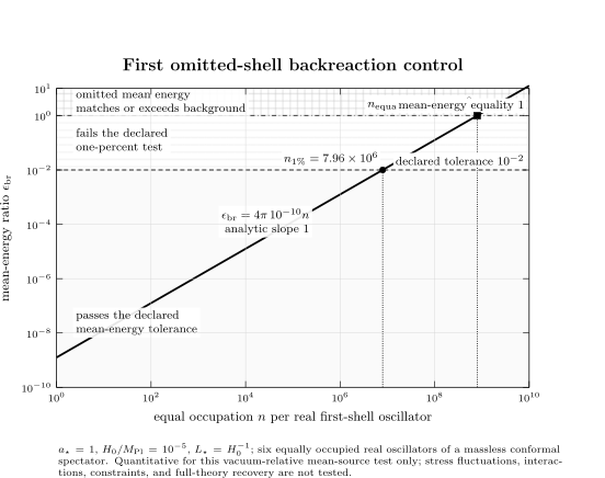
Mean-energy backreaction from the first omitted shell in the declared finite-box benchmark. At $a_\star=1$, $H_0/M_{\mathrm{Pl}}=10^{-5}$, and $L_\star=H_0^{-1}$, equal occupation $n$ of the six real first-shell oscillators gives $\epsilon_{\mathrm{br}}=4\pi n(H_0/M_{\mathrm{Pl}})^2$. The analytic envelope crosses the declared one-percent tolerance at $n=7.9577\times10^6$ and the unavoidable mean-energy failure boundary at $n=7.9577\times10^8$; pure product number states lie at integer $n$. This certifies only the displayed mean-source test, not stress fluctuations, interactions, constraint closure, entanglement, anisotropic sectors, continuum convergence, or full-theory recovery.

Open the full-size figure, download the plotted data, or inspect the semantic record.

Swipe or use the Left and Right arrow keys to inspect every column. Home and End move to the table edges.

Numerical relationships encoded by the omitted-shell backreaction figure

Case	n per oscillator	Total shell quanta	εbr	(H − H0)/H0	Interpretation
Reference vacuum	0	0	0	0	Excitation source vanishes
One quantum each	1	6	1.2566371 × 10−9	6.2831853 × 10−10	Passes this test only
First integer above one percent	7,957,748	47,746,488	0.0100000011	0.0049875626	Fails the declared tolerance
First integer at mean-energy failure	795,774,716	4,774,648,296	1.0000000007	0.4142135626	Homogeneous background split fails

There is no fitted or Monte Carlo uncertainty in this analytic fixture; displayed decimals remain subject to floating-point roundoff and rounding. Its dominant limitation is model dependence: changing $H_0$, the physical box, the state, the field content, or the tested observable changes the threshold. That explicit dependence is a feature, not a defect; it prevents the benchmark from masquerading as a universal bound.

A complete control suite

One small energy ratio is necessary but not sufficient. A publication-level truncation claim should answer every row relevant to its observable.

Question	Diagnostic	Required result
Is the perturbative expansion ordered?	Field amplitudes and an estimate of $S_3/S_2$	Small throughout the claimed domain
Does omitted stress alter the background?	Renormalized energy, pressure, and anisotropic-stress ratios	Below predeclared tolerances
Do omitted oscillators push retained variables?	Vacuum-relative $\sum_I\langle\partial_qH_{2,I}\rangle$ divided by a noncancelling background force scale	Small, state-specified, and stable under adding modes
Are the constraints respected?	Normalized constraint and closure residuals	Of the first omitted order and convergent
Is the answer truncation-stable?	A held-out relational observable under cutoff, basis, and state-space enlargement	Stable within a stated error bar
Is cell invariance genuine?	The same physical state remapped under a $V_0$ change	Intensive observables agree
Is the effective theory applicable?	Curvature and physical momenta compared with its cutoff $\Lambda$	Parametrically below the cutoff

Do not divide a residual by $C_0$: the constraint vanishes on physical solutions. A noncancelling normalization is, for example,

$$r_C= \frac{|\langle C_0+C_2\rangle|} {\sum_A|\langle C_{0,A}\rangle|},$$

where $C_{0,A}$ are the individual gravitational and matter terms. Likewise, an oscillator estimate requires

$$\omega_I^2>0, \qquad \epsilon_{\mathrm{ad},I} =\left|\frac{\omega_I'}{\omega_I^2}\right| \le\tau_{\mathrm{ad}}.$$

If $\omega_I^2\le0$, there is no normalizable instantaneous oscillator ground state. If $\epsilon_{\mathrm{ad},I}$ is order one, particle number is strongly basis-dependent. These failures do not by themselves prove that minisuperspace has failed; they prove that the instantaneous-number estimator has failed. One must instead evolve the mode covariance and compute the renormalized stress directly.

High curvature is a separate obstruction. With the global convention and $N=1$,

$$R=-6(\dot H_{\mathrm{FLRW}}+2H_{\mathrm{FLRW}}^2),$$

and for a flat FLRW metric,

$$K=R_{\mu\nu\rho\sigma}R^{\mu\nu\rho\sigma} =12\left[(\dot H_{\mathrm{FLRW}}+H_{\mathrm{FLRW}}^2)^2 +H_{\mathrm{FLRW}}^4\right].$$

For an effective-theory cutoff $\Lambda$, a useful domain diagnostic is

$$\epsilon_{\mathrm{EFT}} =\max\left\{ \frac{|R|}{\Lambda^2}, \frac{\sqrt K}{\Lambda^2}, \frac{k_{\mathrm{phys}}^2}{\Lambda^2} \right\}.$$

A precision claim needs a declared $\epsilon_{\mathrm{EFT}}$ tolerance. Once this ratio is order one, the derivative expansion has no parametric control even if the minisuperspace equations remain easy to solve.

Three adversarial tests

Excite an anisotropic subset. Instead of populating the symmetric shell, occupy only the two real oscillators associated with the $\pm\hat{\mathbf x}$ pair. In an orthonormal spatial frame, a high-frequency massless excitation has

$$P_{ij}=\operatorname{diag}(\rho,0,0), \qquad \pi_{ij}=\rho\,\operatorname{diag} \left(\frac23,-\frac13,-\frac13\right),$$

so $\sqrt{\pi_{ij}\pi^{ij}}=\sqrt{2/3}\,\rho$. A small mean-energy ratio alone therefore does not certify small shear sourcing. Failure of the anisotropic-stress tolerance downgrades the result to the isotropic state family actually tested.

Change the physical box honestly. If $L_\star$ is doubled while the shell label and $n$ are held fixed, then $k_\star$ halves, the volume grows by eight, and $\Delta\rho_\chi$ falls by sixteen. This is not regulator invariance; it is a different physical wavelength and a different state. A same-state comparison must remap the shell index to keep $k_{\mathrm{phys}}$ fixed and scale the number of occupied modes with volume so that the occupation density is unchanged. Failure after that remapping is genuine cell or coarse-graining dependence.

Approach the edge of the approximation. For a high-frequency massless mode with fixed occupation,

$$\Delta\rho_k\propto a^{-4}.$$

If the background has approximately constant equation-of-state parameter $w$, then $\rho_{\mathrm{bg}}\propto a^{-3(1+w)}$ and

$$\frac{\Delta\rho_k}{\rho_{\mathrm{bg}}} \propto a^{3w-1}.$$

The relative error grows during contraction for $w<1/3$, stays constant for radiation, and decreases for $w>1/3$. “Blue shift implies breakdown” is therefore not universal. Even in the last case, the physical momentum or curvature can cross $\Lambda$ and invalidate the effective theory.

The strongest surviving statement after any failed test is precise: the result remains a property of the finite-dimensional model and of the state, branch, and interval that passed the remaining checks. It is not evidence for stability of the full inhomogeneous theory, and it cannot by itself establish singularity resolution.

Common pitfalls

Exact reduced dynamics is not exact quantum cosmology. Solving every eigenstate of $C_0$ says nothing about the size of $C_2$, $C_3$, or the error in embedding the reduced Hilbert space into the full theory. Approximation control comes from restoring information and testing convergence.

A bare perturbative energy is not renormalized stress. The state, regulator, subtraction prescription, and conservation condition are part of the observable. Vacuum-relative excitation energy is finite, but it does not replace a complete $\langle T_{\mu\nu}\rangle_{\mathrm{ren}}$ calculation.

Small field amplitude need not mean small backreaction. For a high-frequency massless oscillator at fixed occupation, its variance decreases like $1/k$ while its excitation energy grows like $k$. Gradients can be dynamically important even when the field itself looks small.

Changing a mode label is not a same-state cell test. Discrete labels acquire their physical meaning through the box. Transport physical wavelengths and occupation density before comparing intensive predictions.

Exercises

Derive the constraint and Friedmann check

Starting from $S_0$, compute $p_a$, $p_\phi$, and the Hamiltonian constraint. Then recover the Friedmann equation in an arbitrary positive lapse.

Solution

Differentiating the Lagrangian with respect to the velocities gives

$$p_a=-\frac{6M_{\mathrm{Pl}}^2V_0a\dot a}{N}, \qquad p_\phi=\frac{V_0a^3\dot\phi}{N}.$$

Solving for the velocities and evaluating $p_a\dot a+p_\phi\dot\phi-L$ gives $H_{\mathrm{can}}=NC_0$ with

$$C_0=-\frac{p_a^2}{12M_{\mathrm{Pl}}^2V_0a} +\frac{p_\phi^2}{2V_0a^3}+V_0a^3U.$$

Substitute the velocity expressions into $C_0/(V_0a^3)=0$:

$$-3M_{\mathrm{Pl}}^2\left(\frac{\dot a}{Na}\right)^2 +\frac12\left(\frac{\dot\phi}{N}\right)^2+U=0.$$

Therefore $3M_{\mathrm{Pl}}^2H_{\mathrm{FLRW}}^2=\rho_\phi$. The lapse cancels only after the proper-time derivatives are formed.

Reproduce the figure thresholds

Derive $\epsilon_{\mathrm{br}}=4\pi n(H_0/M_{\mathrm{Pl}})^2$ for the six-oscillator shell. Find the first integer $n$ that violates $\tau_\rho=10^{-2}$ and the first that gives $\epsilon_{\mathrm{br}}\ge1$.

Solution

The six oscillators carry vacuum-relative energy $6nk_\star$. Since $k_\star=2\pi/L_\star$ and $L_\star=H_0^{-1}$,

$$\Delta\rho_\chi =\frac{6n(2\pi H_0)}{H_0^{-3}} =12\pi nH_0^4.$$

Dividing by $3M_{\mathrm{Pl}}^2H_0^2$ gives the stated ratio. For $H_0/M_{\mathrm{Pl}}=10^{-5}$,

$$n(\tau)=\frac{\tau}{4\pi\times10^{-10}}.$$

Taking the ceiling gives $n=7{,}957{,}748$ at one percent and $n=795{,}774{,}716$ at unity.

Turn the shell into a shear source

Populate only the $\pm\hat{\mathbf x}$ pair. Subtract the isotropic pressure $P=\rho/3$ from $P_{ij}=\operatorname{diag}(\rho,0,0)$ and compute $\sqrt{\pi_{ij}\pi^{ij}}$.

Solution

The traceless part is

$$\pi_{ij}=P_{ij}-\frac{\rho}{3}\delta_{ij} =\rho\,\operatorname{diag} \left(\frac23,-\frac13,-\frac13\right).$$

Hence

$$\pi_{ij}\pi^{ij} =\rho^2\left(\frac49+\frac19+\frac19\right) =\frac23\rho^2.$$

The anisotropic source is therefore $\sqrt{2/3}\,\rho$. An energy tolerance does not independently test the tensor structure of the stress.

Diagnose the cell trap

Show that doubling the physical box while keeping the first-shell label and occupation fixed sends $\Delta\rho_\chi\to\Delta\rho_\chi/16$. Explain why this is not a violation of fiducial-cell invariance.

Solution

For the first shell, $k\propto L^{-1}$ and $V=L^3$. Thus $k/V\propto L^{-4}$, so $L\to2L$ gives a factor $2^{-4}=1/16$. But the first-shell wavelength has also doubled. The two calculations describe different physical states. A same-state comparison keeps the physical wavelength and occupation density fixed by remapping the discrete shell and increasing the number of occupied modes with the volume.

Test an ultraviolet occupation tail

Suppose an excitation spectrum has $n_k\propto k^{-p}$ at large $k$. In three spatial dimensions, determine when its vacuum-relative energy tail above cutoff $K$ converges.

Solution

The density of modes contributes $k^2\mathrm dk$ and each massless quantum contributes energy proportional to $k$. Therefore

$$\Delta\rho_{>K}\propto \int_K^\infty\mathrm dk\,k^{3-p}.$$

It converges only for $p>4$, when it scales as $K^{4-p}/(p-4)$. It diverges logarithmically for $p=4$ and by a power for $p<4$. Energy convergence is necessary but weaker than the Hadamard and differentiability conditions needed for the full renormalized stress tensor.

Scope and continuations

Minisuperspace is valuable because it isolates constraints, clocks, measures, and boundary proposals in a tractable setting. Its strongest defensible claim is conditional: the reduced result is controlled only over the intersection of the state, mode, tolerance, relational-observable, and effective-theory domains actually tested.

Wheeler–DeWitt Cosmology: Boundary Conditions, Inner Products, and Probabilities quantizes this constraint. Quantum Geometrodynamics Beyond Minisuperspace restores functional degrees of freedom, while BKL, Mixmaster, and Inhomogeneous Singularities tests the homogeneous approximation near spacelike singularities.

The chapter overview contains the structure diagram and validity and failure diagram. They are embedded there once so that their shared chapter-level context is not repeated on every article.

For the chapter-wide comparison of assumptions, counterevidence, falsifiers, and claim ceilings, see the claim-domain table.

References

• Barbero G., J. Fernando, and Eduardo J. S. Villaseñor. “Quantization of Midisuperspace Models.” Living Reviews in Relativity 13 (2010): article 6. DOI.
• Birrell, N. D., and P. C. W. Davies. Quantum Fields in Curved Space. Cambridge Monographs on Mathematical Physics. Cambridge: Cambridge University Press, 1982. DOI.
• Fels, Mark E., and Charles G. Torre. “The Principle of Symmetric Criticality in General Relativity.” Classical and Quantum Gravity 19 (2002): 641–675. DOI; arXiv.
• Halliwell, J. J., and S. W. Hawking. “Origin of Structure in the Universe.” Physical Review D 31 (1985): 1777–1791. DOI.
• Mele, Fabio M., and Johannes Münch. “On the Role of Fiducial Structures in Minisuperspace Reduction and Quantum Fluctuations in LQC.” Classical and Quantum Gravity 41 (2024): 245003. DOI; arXiv.
• Mukhanov, Viatcheslav F., H. A. Feldman, and Robert H. Brandenberger. “Theory of Cosmological Perturbations.” Physics Reports 215 (1992): 203–333. DOI.
• Schander, Susanne, and Thomas Thiemann. “Quantum Cosmological Backreactions. IV. Constrained Quantum Cosmological Perturbation Theory.” Physical Review D 105 (2022): 106012. DOI; arXiv.