Microstate Geometries and Fuzzball Proposals

Microstate geometries are controlled classical solutions that make one part of black-hole microphysics geometrically visible: topology and flux replace a horizon and singular source while the exterior carries black-hole charges. Their existence is a major constructive result. It is not, by itself, evidence that every black-hole microstate is a smooth geometry, that the known families contain $e^{S_{\rm BH}}$ independent states, or that a typical nonextremal state has a classical cap.

This page therefore separates five increasingly strong statements: a candidate solves the local BPS equations; it is globally smooth and causal; it represents an identifiable quantum state or coherent-state family; its quantization supplies an entropy-sized set; and that set is typical for specified observables and a specified measure. We develop the first two questions in a five-dimensional BPS model, test a three-center scaling candidate, and then compare the known superstratum count with the BMPV entropy.

Required background. D-Brane Bound States and the Strominger–Vafa Count fixes the microscopic charge sector; Attractor Mechanism and Charge-Only Entropy fixes the near-horizon target.

Helpful background. Wormholes, Chronology, and Superluminal-Travel Constraints supplies causal regularity tests; Evidence Independence, Circularity, and Double Counting supplies the evidence boundary.

Evidence cutoff: 29 August 2026. The construction formulas below are stable results. Statements about how much of the black-hole Hilbert space is represented by known families are dated research assessments.

Microstate geometries and the fuzzball claim

A fuzzball is a proposed individual black-hole microstate whose horizon-scale physics differs substantially from the vacuum-horizon description. It need not admit a classical metric. A microstate geometry is the much more restrictive semiclassical case: a smooth, horizonless supergravity solution, normally with the same conserved charges and asymptotic boundary conditions as a black hole, that is argued to represent a state or coherent superposition in the corresponding quantum theory. The distinction matters because a classical field profile is naturally closer to a coherent state than to a generic energy eigenstate Mayerson 2022, §1.2, pp. 6–8.

For a useful claim, four labels should accompany the words “microstate geometry”:

• the compactification and lower-dimensional effective theory;
• the asymptotic boundary conditions and conserved-charge sector;
• the amount of supersymmetry and the regime in which supergravity is controlled;
• the evidence that connects the classical solution to a quantum state.

The worked construction uses the following model card.

Item	Declaration
Theory	Ungauged five-dimensional $\mathcal N=2$ STU supergravity with three Abelian gauge fields
Origin	A standard truncation of M-theory on $T^6$, dualizable to a D1–D5–P frame
Couplings	$C_{IJK}=\lvert\epsilon_{IJK}\rvert$, with $I,J,K=1,2,3$
Asymptotics	Five-dimensional asymptotic flatness; the later superstratum comparison instead uses an $AdS_3\times S^3$ decoupling region
Signature	The site’s mostly-minus Lorentzian convention; the Gibbons–Hawking base is written with positive spatial line element where $V>0$
Classical control	Curvature radii and flux-supported cycles must remain large compared with the appropriate Planck and string scales
Quantum claim	None follows from the ansatz alone; a state map, symplectic form, and quantization are additional inputs

The preceding localization article studies a fixed-charge horizon functional. Here the observable is different: an explicit classical configuration and the data needed to decide whether it belongs to a controlled quantum family.

BPS data on a Gibbons–Hawking base

The supersymmetric construction becomes a sequence of linear equations on a four-dimensional base. Let $\vec x\in\mathbb R^3$, let the coordinate $\psi$ have period $4\pi$, and write

$$ds_4^2 =V^{-1}(d\psi+A)^2+V\,d\vec x^{\,2}, \qquad \vec\nabla\times\vec A=\vec\nabla V .$$

The complete five-dimensional metric is

$$ds_5^2 =Z^{-2}(dt+k)^2-Z\,ds_4^2, \qquad Z=(Z_1Z_2Z_3)^{1/3}.$$

Eight harmonic functions on $\mathbb R^3$ determine the solution:

$$H=(V,K^I,L_I,M) =h+\sum_{a=1}^{n_c}\frac{\Gamma_a}{r_a}, \qquad r_a=\lvert\vec x-\vec x_a\rvert,$$

with center data

$$\Gamma_a=(v_a,k_a^I,\ell_{Ia},m_a).$$

Here $v_a$ is a Gibbons–Hawking residue, not an asymptotic electric charge. The remaining fields are assembled as

$$Z_I =L_I+\frac12 C_{IJK}\frac{K^J K^K}{V},$$ $$\mu =M+\frac{K^I L_I}{2V} +\frac16 C_{IJK}\frac{K^I K^J K^K}{V^2}, \qquad k=\mu(d\psi+A)+\omega,$$

and

$$\vec\nabla\times\vec\omega =V\vec\nabla M-M\vec\nabla V +\frac12\left(K^I\vec\nabla L_I-L_I\vec\nabla K^I\right).$$

These formulas are the five-dimensional BPS hierarchy in harmonic form Bena and Warner 2006, §3.1, Eqs. (3.5), (3.12)–(3.17). They solve the local supersymmetry equations, but arbitrary harmonic residues need not produce a smooth or causal spacetime.

Local cancellation at a center

Suppose $v_a\ne0$. Requiring the apparent poles in $Z_I$ and $\mu$ to cancel fixes

$$\ell_{Ia} =-\frac12 C_{IJK}\frac{k_a^Jk_a^K}{v_a}, \qquad m_a =\frac1{12}C_{IJK} \frac{k_a^Ik_a^Jk_a^K}{v_a^2}.$$

For $\lvert v_a\rvert=1$, the $\psi$ fiber can pinch off smoothly at an isolated center; larger integral $\lvert v_a\rvert$ generally gives a local orbifold unless further structure resolves it. Some useful bases are ambipolar: $V$ changes sign. The base metric then changes signature, but the factors in the full five-dimensional metric can cancel the apparent singularity. Testing only the base would therefore reject valid solutions; testing only the pole cancellation would accept invalid ones.

The local relations, the harmonic hierarchy, and the regularity conditions are derived together in Mayerson 2022, §2.2–§2.4, pp. 14–19. They are a convenient starting point, not a global existence theorem.

Flux cycles, bubble equations, and the causal gate

Between centers $a$ and $b$, the $\psi$ fiber over a path in $\mathbb R^3$ forms a topological two-sphere. Its gauge-invariant magnetic flux is proportional to

$$\Pi_{ab}^{I} =\frac{k_b^I}{v_b}-\frac{k_a^I}{v_a}.$$

The flux supports the cycle against collapse. Under the harmonic gauge shift $k_a^I\mapsto k_a^I+c^Iv_a$, each ratio shifts by the same $c^I$, so $\Pi_{ab}^{I}$ is unchanged. This is why the individual $k_a^I$ are not themselves physical fluxes Mayerson 2022, §2.6, Eq. (37), pp. 20–21.

In the convention used below, define

$$\langle\Gamma,\Gamma'\rangle =2(vm'-mv')+k^I\ell'_I-\ell_Ik'^I .$$

Removing Dirac–Misner strings from $\omega$, equivalently requiring $\mu$ to vanish appropriately at the centers, gives the bubble equations

$$\sum_{b\ne a} \frac{\langle\Gamma_a,\Gamma_b\rangle}{r_{ab}} =\langle h,\Gamma_a\rangle, \qquad r_{ab}=\lvert\vec x_a-\vec x_b\rvert .$$

Only $n_c-1$ of these equations are independent because the sum of their left-hand sides vanishes. They are necessary integrability conditions. They do not prove the absence of closed timelike curves.

Two central algebraic inequalities are

$$VZ_I\ge0 \quad\text{for each }I, \qquad \mathcal Q \equiv Z_1Z_2Z_3V-\mu^2V^2\ge0,$$

throughout the spacetime. A full check must also control $\omega$, the norms of compact angular orbits, the neighborhoods of every center, the $V=0$ surfaces, infinity, and the curvature scale Bena and Warner 2006, §3.2 and §4.4. A grid with positive values is evidence, not a proof over a continuum.

Harmonic residues are not five-dimensional electric charges

For $n_c$ smooth centers and five-dimensional asymptotic flatness, set

$$\bar k^I=\frac1{n_c}\sum_a k_a^I, \qquad \widetilde k_a^I=k_a^I-n_c v_a\bar k^I .$$

In the gauge and normalization of Bena, Wang, and Warner 2006, §2.2, Eqs. (2.21)–(2.26), the electric charges measured at infinity and the two angular momenta are

$$Q_I =-2C_{IJK}\sum_a \frac{\widetilde k_a^J\widetilde k_a^K}{v_a},$$ $$J_R =\frac43C_{IJK}\sum_a \frac{\widetilde k_a^I\widetilde k_a^J\widetilde k_a^K}{v_a^2}, \qquad \vec J_L=8\vec D, \qquad \vec D=\sum_{a,I}\widetilde k_a^I\vec x_a.$$

The quadratic and cubic dependence is a Chern–Simons/flux effect. Thus $\sum_a\Gamma_a$ is the total harmonic residue, not a synonym for the physical five-dimensional charge vector. Factors in these formulas vary across the literature; a numerical result is meaningless unless its convention accompanies it.

Worked check: a three-center scaling candidate

The purpose of this example is not to announce a new microstate geometry. It is to show how far exact algebra takes us and where a global proof is still required.

Take three centers with the following residues:

$a$	$v_a$	$(k_a^1,k_a^2,k_a^3)$	$(\ell_{1a},\ell_{2a},\ell_{3a})$	$m_a$
1	$1$	$(0,0,0)$	$(0,0,0)$	$0$
2	$1$	$(-1,-1,3)$	$(3,3,-1)$	$3/2$
3	$-1$	$(2,2,-1)$	$(-2,-2,4)$	$-2$

The $\ell_{Ia}$ and $m_a$ entries follow exactly from the local cancellation formulas. The oriented cycle-flux vectors are

$$\vec\Pi_{12}=(-1,-1,3), \qquad \vec\Pi_{23}=(-1,-1,-2), \qquad \vec\Pi_{31}=(2,2,-1),$$

where each vector groups the three values of $I$. Thus the flux data are integral in this normalization. Since $\sum_av_a=1$, the Gibbons–Hawking base approaches $\mathbb R^4$. Choose

$$h=(0;0,0,0;1,1,1;-2),$$

so that

$$\begin{aligned} V&=\frac1{r_1}+\frac1{r_2}-\frac1{r_3},\\ K^1=K^2&=-\frac1{r_2}+\frac2{r_3}, &K^3&=\frac3{r_2}-\frac1{r_3},\\ L_1=L_2&=1+\frac3{r_2}-\frac2{r_3}, &L_3&=1-\frac1{r_2}+\frac4{r_3},\\ M&=-2+\frac{3}{2r_2}-\frac2{r_3}. \end{aligned}$$

The constant $m_0=-2$ makes $\mu$ vanish at infinity in this gauge.

Exact bubble-equation solution

The oriented products and source terms are

$$\bigl( \langle\Gamma_1,\Gamma_2\rangle, \langle\Gamma_2,\Gamma_3\rangle, \langle\Gamma_3,\Gamma_1\rangle \bigr) =(3,2,4),$$ $$\bigl( \langle h,\Gamma_1\rangle, \langle h,\Gamma_2\rangle, \langle h,\Gamma_3\rangle \bigr) =(4,3,-7).$$

Hence the three equations reduce to

$$\frac3{r_{12}}-\frac4{r_{13}}=4, \qquad -\frac3{r_{12}}+\frac2{r_{23}}=3, \qquad \frac4{r_{13}}-\frac2{r_{23}}=-7.$$

Writing $x=3/r_{12}$ gives the exact one-parameter family

$$r_{12}=\frac3x, \qquad r_{13}=\frac4{x-4}, \qquad r_{23}=\frac2{x+3}.$$

Substitution makes the residuals transparent:

$$x-(x-4)=4, \qquad -x+(x+3)=3, \qquad (x-4)-(x+3)=-7.$$

Positive distances require $x>4$. The only nonautomatic triangle inequality is $r_{12}+r_{23}>r_{13}$, which becomes

$$x^2-23x-36>0,$$

so a genuine triangle exists when

$$x>x_{\rm crit} =\frac{23+\sqrt{673}}2 \simeq24.471.$$

With $\lambda=1/x$, the center separations scale as

$$\begin{aligned} r_{12}&=3\lambda,\\ r_{13}&=4\lambda+16\lambda^2+O(\lambda^3),\\ r_{23}&=2\lambda-6\lambda^2+O(\lambda^3). \end{aligned}$$

The leading shape therefore has $r_{12}:r_{13}:r_{23}=3:4:2$. Its strict triangle inequalities hold. This is stronger than merely postulating compatible pairings: the full center residues and the inhomogeneous bubble equations are explicit.

Charges and angular momenta

The gauge-invariant shifted residues are

$$\widetilde k_1=(-1,-1,-2), \qquad \widetilde k_2=(-2,-2,1), \qquad \widetilde k_3=(3,3,1).$$

They give

$$(Q_1,Q_2,Q_3)=(12,12,16), \qquad J_R=88,$$

and the BMPV discriminant in this normalization is positive:

$$Q_1Q_2Q_3-\frac{J_R^2}{4}=368>0.$$

Place $\vec x_1=0$, $\vec x_2=(r_{12},0,0)$, and $\vec x_3=(u,v,0)$ with the distances above. The second angular momentum is

$$\lvert J_L\rvert =8\sqrt{-12r_{12}^2+28r_{13}^2+21r_{23}^2} =16\sqrt{106}\,\lambda+O(\lambda^2).$$

Thus $Q_I$ and $J_R$ remain fixed along the family, while $J_L$ tends to zero rather than remaining exactly fixed at finite $\lambda$. At $x=100$, for example,

$$(r_{12},r_{13},r_{23}) \simeq(0.0300,0.04167,0.01942), \qquad \lvert J_L\rvert\simeq1.711.$$

What passes, and what does not

Check	Result	Status
Integral GH residues, cycle fluxes, and local pole cancellation	Exact for all three centers and all three oriented cycles	Passed locally
Bubble equations	All three residuals vanish algebraically	Passed
Triangle geometry	Exists for $x>x_{\rm crit}$	Passed
Asymptotic $Q_I$ and $J_R$	$(12,12,16)$ and $88$	Passed in the declared normalization
Scaling hierarchy	$r_{ab}=\lambda\rho_{ab}+O(\lambda^2)$	Passed classically
Global $VZ_I$ and $\mathcal Q$ positivity	Deterministic sampling found no negative point, but does not cover the continuum	Supportive, not certified
Regularity of $\omega$ and every angular orbit	Not proved over the complete domain	Open
Quantum-state map and count	Not supplied by the classical fixture	Open

A deterministic reconnaissance sampled $500{,}000$ points at each of $x=25,30,50,100,200,1000$. For each $x$, a seeded linear-congruential generator chose directions uniformly on the sphere about the center-of-position centroid and radii log-uniformly from $10^{-3}$ to $10^3$ times the largest intercenter separation; the seed was $123456789+x$. No sampled point had negative $VZ_I$ or $\mathcal Q$. This broad scan does not deliberately target the center neighborhoods or the $V=0$ surfaces. Very near a center, moreover, the separate terms in $\mathcal Q$ scale as high inverse powers and suffer severe floating-point cancellation. A publication-grade certification would need analytic patches at every center, infinity, and each $V=0$ surface, followed by interval subdivision of the remaining compact domain and a regular construction of $\omega$.

Verdict. This is a locally regular, flux-quantized scaling candidate with exact bubble equations and controlled asymptotic charges. It is not called a microstate geometry here because the global causal gate has not been certified. The failed promotion is part of the result, not a defect to hide.

A deep throat ending in a finite cap

Why does a shrinking coordinate cluster resemble a black hole more closely from far away? In the intermediate region

$$r_{ab}\ll r\ll r_{\rm mouth},$$

the separate harmonic poles are unresolved and the cluster looks approximately like one charged center. The radial metric has the throat form

$$ds_{\rm rad}^2 \simeq R_{\rm th}^2\frac{dr^2}{r^2},$$

where $R_{\rm th}$ is fixed by the asymptotic charges—proportional to $(Q_1Q_2Q_3)^{1/6}$ in the usual five-dimensional normalization. If $r_{\rm cap}=c\lambda$ for a fixed conversion scale $c$, then

$$L_{\rm th}(\lambda) \simeq R_{\rm th} \log\!\left(\frac{r_{\rm mouth}}{c\lambda}\right).$$

The comparison between two configurations is free of the convention-dependent constant:

$$\Delta L_{\rm th} =L_{\rm th}(\lambda_2)-L_{\rm th}(\lambda_1) =R_{\rm th}\log\!\left(\frac{\lambda_1}{\lambda_2}\right), \qquad 0<\lambda_2<\lambda_1.$$

This logarithm is a proper length, not coordinate time and not a trajectory in which centers dynamically fall together. At every finite $\lambda$, a globally regular scaling solution has a finite redshift and ends in a flux-supported cap. The classical $\lambda\to0$ endpoint lies at a boundary of configuration space; it cannot be counted as an infinite continuum of quantum states Bena, Wang, and Warner 2006, §3–§4, Warner 2019, §§4.8 and 5.

The figure shows the spatial relation to inspect: the fibered cycles persist while their coordinate presentation shrinks, and the exterior develops a longer unresolved throat. It depicts the mechanism conditional on passing the global causal gate; it does not upgrade the worked candidate’s status.

On a narrow screen, swipe or use the Left and Right arrow keys to pan across the figure. Home and End move to its edges. A full-size link is also available.

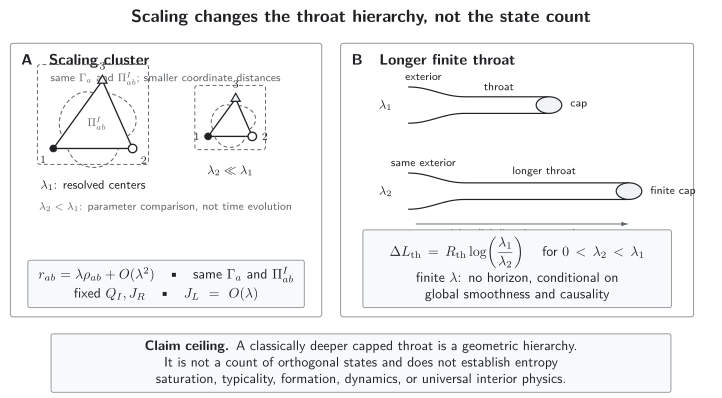
The three-center configurations differ by the scaling parameter, not by time evolution. The discrete center and flux data keep $Q_I$ and $J_R$ fixed in the worked family, while $r_{ab}=\lambda\rho_{ab}+O(\lambda^2)$ and $J_L=O(\lambda)$. Reducing $\lambda$ adds the quantitative proper length $\Delta L_{\rm th}=R_{\rm th}\log(\lambda_1/\lambda_2)$ before a finite-$\lambda$ flux-supported cap, provided the global smoothness and no-closed-timelike-curve conditions hold. The cluster shapes, throat profiles, and sizes are schematic and not to scale. Neither depth nor smoothness is a state count or a typicality result.

Feature	Along the worked scaling family
Fixed	Center residues, cycle fluxes, $Q_I$, $J_R$, and asymptotic moduli
Changes	Coordinate separations, redshift hierarchy, proper throat length, and $J_L=O(\lambda)$
Finite-$\lambda$ endpoint	A cap, provided the global smoothness and causal conditions hold
Does not follow	A count of orthogonal states, entropy completeness, typicality, formation, or universal interior physics

From a classical family to quantum states

A continuous family of classical solutions is not a continuum of orthogonal states. Suppose a regular reduced moduli space $\mathcal M_{\rm reg}$ has dimension $2n$ and symplectic form $\Omega$. When the space, boundary conditions, gauge quotient, and semiclassical approximation are controlled, its leading phase-space count is schematically

$$N_{\rm geom} \simeq\frac1{(2\pi\hbar)^n} \int_{\mathcal M_{\rm reg}}\frac{\Omega^n}{n!}, \qquad S_{\rm geom}=\log N_{\rm geom}.$$

Every noun in this expression matters. Singular boundaries can change the quantization; noncompact directions can make the integral diverge; gauge-equivalent points must not be counted twice; and a coherent-state parametrization may overcount linearly dependent quantum states.

For multicenter BPS solutions, the symplectic form inherited from the full theory has been quantized in controlled sectors. In the studied three-center scaling case, the quantum wavefunctions suppress the classically infinite-throat boundary rather than furnishing infinitely many ever-deeper orthogonal states de Boer et al. 2009, §3.2.1, §4, and §8. This is an important mechanism, not a theorem about every superstratum or non-BPS family.

A holographic state map is a second, independent bridge. The two-charge Lunin–Mathur profiles have a particularly controlled map to D1–D5 Ramond ground states and a semiclassical phase-space quantization Lunin and Mathur 2002, §4–§6; Rychkov 2006, §2.1–§2.2. Quantizing the four transverse bosonic profile modes gives

$$\log\Gamma_{\rm profile} \sim2\pi\sqrt{\frac23N_1N_5},$$

which recovers the $\sqrt{N_1N_5}$ growth but not the full $T^4$ coefficient $2\pi\sqrt{2N_1N_5}$; internal and fermionic sectors supply additional states. Many three-charge superstrata similarly map to coherent combinations of protected CFT excitations. Such a map identifies a controlled family, but orthogonality, completeness, and a measure over the entire finite-area black-hole sector remain separate questions. See D1–D5 CFT and AdS₃ Microstate Data for the state dictionary and BPS Indices, Absolute Degeneracies, and Wall Crossing for the distinction between an index and an absolute count.

Which solution families establish which claims

The families below solve different problems. They should not be pooled into one undifferentiated “number of fuzzballs.”

Family	Controlled setting	State and count evidence	Strongest licensed claim	Principal limitation
Lunin–Mathur profiles	Smooth two-charge D1–D5 geometries; asymptotically flat or $AdS_3\times S^3$ decoupling limit	Detailed CFT profile map and semiclassical quantization	A large, controlled geometric realization of the two-charge ground-state sector	The two-charge system has no macroscopic five-dimensional horizon; a generic exact state need not be one classical profile
GH multicenters	Five-dimensional BPS solutions supported by fluxed two-cycles	Explicit families and reduced phase-space quantization in selected sectors	Smooth horizonless solutions with black-hole charges and controllably deep throats exist	Known counts are not entropy-saturating; global no-CTC and scaling-boundary control are family-specific
Superstrata	Six-dimensional BPS D1–D5–P solutions, commonly in $AdS_3\times S^3$	Mode-by-mode CFT/coherent-state maps and direct symplectic quantization for important families	Vast functional three-charge families with controlled regularity and state data exist	The known empty-$AdS_3\times S^3$ families are parametrically sub-entropic
Vector superstrata	Six-dimensional extensions with vector multiplets	Explicit regular solutions and coherent-state interpretations for selected modes	Additional matter sectors can support finite long-throat microstructure	Completeness, full quantization, generic stability, and entropy saturation are open
Microstrata	Non-BPS six-dimensional and Type-IIB solutions obtained through a consistent three-dimensional truncation, asymptotic to $AdS_3\times S^3\times T^4$	Coherent left- and right-moving D1–D5 interpretation plus perturbative and numerical nonlinear solutions	Controlled non-BPS caps exist inside the stated truncation and boundary conditions	Asymptotically flat completion, decay, long-time stability, and entropy count remain open
Q-ball proof of concept	Selected non-BPS modes in the same $AdS_3$-based truncation	Perturbative solution data; some modes develop non-normalizable pieces	Supersymmetry is not logically required for every capped construction	Boundary-condition admissibility and generic state, stability, and counting claims do not follow

The two-charge result is reviewed technically in Mayerson 2022, §3.2–§3.3, pp. 23–27, while the original constructive superstratum argument appears in Bena et al. 2015, §§2–6. Recent extensions include Ganchev et al. 2023, §1 and §7, Čeplak and Hampton 2024, and the proof-of-concept Ganchev, Houppe, and Warner 2021. Time-dependent microstrata move away from the special locus perturbatively, but unresolved secular terms limit long-time control Houppe 2024, §4 and §6; the six-dimensional uplift of a simple special-locus construction sharpens the dictionary without establishing generic stability or asymptotically flat non-BPS families Ramella and Warner 2026, §3–§5.

Current program reviews emphasize both the size of the six-dimensional solution space and the still-parametric entropy deficit of counted families; fully localized ten- and eleven-dimensional constructions remain under development Bena et al. 2022, §§1 and 6, Bena and Warner 2026, chapter 29, pp. 268–278.

Stability is not a binary label for the entire program. For particular asymptotically flat supersymmetric microstate geometries, stable trapping implies extremely slow wave decay; a nonlinear instability is a serious heuristic expectation, not a proved universal theorem Eperon, Reall, and Santos 2016, §1–§2. Rigorous scalar-wave results prove boundedness in the studied backgrounds while also establishing nondecay or severe decay obstructions in relevant sectors Keir 2020, Theorems 4.6, 4.15, and 5.1. These results constrain those geometries; they do not establish either generic stability or generic instability of capped solutions.

Known-family counting versus BMPV entropy

An explicit entropy comparison prevents a large classical function space from being mistaken for a complete Hilbert space. Let

$$N=N_1N_5$$

for the D1–D5 CFT, take $J=0$, and enter the Cardy regime $N_p\gg N\gg1$. The three-charge BMPV entropy scales as

$$S_{\rm BMPV}=2\pi\sqrt{NN_p} \sim N^{1/2}N_p^{1/2}.$$

The quantized superstrata constructed as nonlinear excitations above empty $AdS_3\times S^3$ instead have the parametric growth

$$S_{\rm known\ strata} \sim N^{1/2}N_p^{1/4}.$$

Therefore

$$\frac{S_{\rm known\ strata}}{S_{\rm BMPV}} \sim N_p^{-1/4}\longrightarrow0.$$

The number of represented states is smaller than the black-hole count by an exponential factor of order

$$\exp\!\left(S_{\rm known\ strata}-S_{\rm BMPV}\right).$$

This conclusion was obtained from the CFT/supergraviton count Shigemori 2019, Eqs. (1.1)–(1.4), §4.6 and independently reproduced by direct supergravity phase-space quantization Mayerson and Shigemori 2021, §4. It rules out entropy saturation and microcanonical typicality for that counted family in that regime. It does not rule out fractional modes, different backgrounds, more stringy states, or families not yet constructed.

To state typicality operationally, choose an ensemble $\mathcal H_Q$, a normalized measure $\mu$, and an observable $\mathcal O$. A concentration claim has the form

$$\mu\!\left( \left\{\psi\in\mathcal H_Q: \lvert\mathcal O(\psi)-\langle\mathcal O\rangle_{\rm micro}\rvert >\varepsilon\right\} \right)\ll1.$$

“Complicated,” “deep,” and “black-hole-like from far away” are not substitutes for this statement. Critical analyses have stressed precisely this gap between constructing smooth examples and demonstrating a typical ensemble Raju and Shrivastava 2019. The constructive and critical arguments test different links in the inference chain; neither should be omitted.

Evidence ceilings and failure tests

Read this ladder cumulatively: each row assumes that the earlier geometric and evidentiary gates have also passed.

Evidence obtained	Strongest conclusion	What is still missing
Local BPS solution and pole cancellation	A regular center candidate	Global causality, flux quantization, and asymptotic control
Quantized flux, bubble equations, complete local regularity, asymptotics, global no-CTC tests, and curvature control	A smooth causal classical geometry in the declared theory and regime	A quantum-state identification
Matching $Q_I$, angular momenta, and boundary conditions	Membership in the same conserved-charge sector	Orthogonality, completeness, and a measure
CFT or coherent-state map	Identified controlled states or state families	An entropy-sized count
Phase-space quantization	A count for the specified reduced phase space	Proof that the phase space is complete
Entropy-sized count	Sufficient cardinality in that ensemble	Typical observables, stability, formation, and dynamics

The strongest current conclusion is therefore deliberately asymmetric. Explicit smooth horizonless solutions, topological support by flux, deep finite throats, and detailed state maps exist in important supersymmetric sectors. No known geometric family has yet supplied a controlled measure over the full $e^{S_{\rm BH}}$ state space of a finite-area three-charge or generic nonextremal black hole, and the known superstratum count is parametrically smaller than the relevant entropy.

Common pitfalls

Equating the bubble equations with causality. The bubble equations remove a local integrability obstruction and constrain center separations. They do not replace the global $VZ_I$, $\mathcal Q$, $\omega$, angular-orbit, and curvature checks.

Calling $\sum_a\Gamma_a$ the five-dimensional charge. It is the total harmonic residue. Chern–Simons couplings make the physical electric charges quadratic in gauge-invariant flux data.

Counting the scaling parameter as states. The classical variable $\lambda$ labels a direction in configuration space. Quantization can cap or suppress the infinite-throat boundary; an uncountable classical family is not an infinite entropy.

Using smoothness as evidence of typicality. Smoothness is a local and global geometric property. Typicality requires a state space, measure, observables, and concentration estimate.

Generalizing a family-specific instability. An unstable mode is decisive for the stated background and perturbation class. It is not evidence that all horizonless solutions share the same spectrum.

Exercises

1. Gauge-invariant cycle flux

Under

$$k_a^I\mapsto k_a^I+c^Iv_a,$$

show that $\Pi_{ab}^I$ is invariant. Explain why it is safer to label a bubble by $\Pi_{ab}^I$ than by either endpoint residue.

Solution

Each endpoint ratio transforms as

$$\frac{k_a^I}{v_a}\mapsto\frac{k_a^I}{v_a}+c^I.$$

The common shift cancels in the difference:

$$\Pi_{ab}^I \mapsto \left(\frac{k_b^I}{v_b}+c^I\right) -\left(\frac{k_a^I}{v_a}+c^I\right) =\Pi_{ab}^I.$$

The flux is therefore invariant under this redundancy, whereas the individual $k_a^I$ are gauge-dependent bookkeeping data.

2. Exact scaling residuals

For the worked family, substitute

$$r_{12}=\frac3x, \qquad r_{13}=\frac4{x-4}, \qquad r_{23}=\frac2{x+3}$$

into the bubble equations. Then determine the leading scaling shape as $x\to\infty$.

Solution

The three left-hand sides are

$$\frac3{r_{12}}-\frac4{r_{13}} =x-(x-4)=4,$$ $$-\frac3{r_{12}}+\frac2{r_{23}} =-x+(x+3)=3,$$

and

$$\frac4{r_{13}}-\frac2{r_{23}} =(x-4)-(x+3)=-7.$$

Thus every residual vanishes exactly. With $\lambda=1/x$,

$$r_{12}:r_{13}:r_{23}\longrightarrow3:4:2.$$

All strict triangle inequalities hold for the limiting shape. This establishes an exact integrable scaling family, not global causal regularity.

3. Logarithmic throat length

Given

$$ds_{\rm rad}^2=R_{\rm th}^2\frac{dr^2}{r^2},$$

integrate from $r_{\rm cap}=c\lambda$ to a fixed $r_{\rm mouth}$. How much longer is the throat when $\lambda_1$ is replaced by the smaller $\lambda_2$?

Solution

The proper length is

$$L_{\rm th}(\lambda) =\int_{c\lambda}^{r_{\rm mouth}} R_{\rm th}\frac{dr}{r} =R_{\rm th}\log\!\left( \frac{r_{\rm mouth}}{c\lambda} \right).$$

Subtracting cancels the arbitrary matching scale $c$ and the fixed mouth radius:

$$L_{\rm th}(\lambda_2)-L_{\rm th}(\lambda_1) =R_{\rm th}\log\!\left(\frac{\lambda_1}{\lambda_2}\right)>0.$$

No horizon occurs at finite $\lambda$ if the full geometry is smooth and causal. The divergence occurs only at the classical boundary $\lambda=0$.

4. Necessary is not sufficient

A numerical fixture has integral fluxes, exact local pole cancellation, and bubble-equation residuals below $10^{-12}$. At one sampled point, however, a compact angular orbit has negative spatial norm and becomes timelike. What claim survives?

Solution

The configuration fails the global causal gate and must be rejected as a microstate geometry. The surviving statement is only that the harmonic data define a locally regular, integrable candidate with the declared charges. Smaller bubble residuals cannot repair a closed timelike curve because the two tests answer different questions.

5. Entropy adversary

In the regime $N_p\gg N\gg1$, compare

$$S_{\rm known}\sim N^{1/2}N_p^{1/4} \qquad\text{and}\qquad S_{\rm BH}\sim N^{1/2}N_p^{1/2}.$$

What does the comparison show, and what does it leave open?

Solution

The entropy ratio is

$$\frac{S_{\rm known}}{S_{\rm BH}} \sim N_p^{-1/4}\to0.$$

If the two counts refer to the same charge sector, the fraction of states represented by the known family is exponentially small, of order $\exp(S_{\rm known}-S_{\rm BH})$. The family is therefore not entropy-saturating or microcanonically typical in this regime. The result does not exclude other superstrata backgrounds, fractional modes, string-scale states, or geometric families not yet known.

What the geometry evidence establishes

Microstate-geometry research has established a concrete mechanism—topological cycles supported by quantized flux—for constructing smooth horizonless configurations with black-hole charges. It has also produced controlled two-charge state maps, large three-charge BPS families, finite scaling throats, selected phase-space quantizations, and special non-BPS extensions. These are substantial results about the existence and structure of black-hole microphysics.

The evidence does not yet establish that a generic black-hole microstate is a smooth metric, that known classical families account for the full finite-area entropy, or that their morphology determines generic absorption, emission, formation, or interior experience. Next, test normalized response rather than morphology alone in Absorption, Emission, and Dynamical Tests; then combine geometry, counting, and dynamics in Typicality, Non-BPS Extensions, and Evidence Limits.

The chapter overview contains the structure diagram and validity and failure diagram. They are embedded there once so that their shared chapter-level context is not repeated on every article.

For the chapter-wide comparison of assumptions, counterevidence, falsifiers, and claim ceilings, see the claim-domain table.

References

• Bena, Iosif, Stefano Giusto, Rodolfo Russo, Masaki Shigemori, and Nicholas P. Warner. “Habemus Superstratum! A Constructive Proof of the Existence of Superstrata.” Journal of High Energy Physics 2015, 5 (2015): 110. DOI. Open PDF.
• Bena, Iosif, Emil J. Martinec, Samir D. Mathur, and Nicholas P. Warner. “Fuzzballs and Microstate Geometries: Black-Hole Structure in String Theory.” Journal of High Energy Physics 2022, 11 (2022): 031. DOI. Open PDF.
• Bena, Iosif, Chih-Wei Wang, and Nicholas P. Warner. “Mergers and Typical Black Hole Microstates.” Journal of High Energy Physics 2006, 11 (2006): 042. DOI. Open PDF.
• Bena, Iosif, and Nicholas P. Warner. “Bubbling Supertubes and Foaming Black Holes.” Physical Review D 74 (2006): 066001. DOI. Open PDF.
• Bena, Iosif, and Nicholas P. Warner. “Microstate Geometries.” In Half a Century of Supergravity, chapter 29, 268–278. Cambridge University Press, 2026. DOI. Open preprint.
• Čeplak, Nejc, and Shaun D. Hampton. “Vector Superstrata: Part Two.” Journal of High Energy Physics 2024, 10 (2024): 011. DOI. Open PDF.
• de Boer, Jan, Frederik Denef, Sheer El-Showk, Ilies Messamah, and Dieter Van den Bleeken. “Quantizing $\mathcal N=2$ Multicenter Solutions.” Journal of High Energy Physics 2009, 5 (2009): 002. DOI. Open PDF.
• Eperon, Felicity C., Harvey S. Reall, and Jorge E. Santos. “Instability of Supersymmetric Microstate Geometries.” Journal of High Energy Physics 2016, 10 (2016): 031. DOI. Open PDF.
• Ganchev, Bogdan, Stefano Giusto, Anthony Houppe, Rodolfo Russo, and Nicholas P. Warner. “Microstrata.” Journal of High Energy Physics 2023, 10 (2023): 163. DOI. Open PDF.
• Ganchev, Bogdan, Anthony Houppe, and Nicholas P. Warner. “Q-Balls Meet Fuzzballs: Non-BPS Microstate Geometries.” Journal of High Energy Physics 2021, 11 (2021): 028. DOI. Open PDF.
• Houppe, Anthony. “Time-Dependent Microstrata in $AdS_3$.” Journal of High Energy Physics 2024, 9 (2024): 083. DOI. Open PDF.
• Keir, Joe. “Wave Propagation on Microstate Geometries.” Annales Henri Poincaré 21 (2020): 705–760. DOI. Open PDF.
• Lunin, Oleg, and Samir D. Mathur. “AdS/CFT Duality and the Black Hole Information Paradox.” Nuclear Physics B 623 (2002): 342–394. DOI. Open PDF.
• Mayerson, Daniel R. “Modave Lectures on Horizon-Size Microstructure, Fuzzballs and Observations.” SciPost Physics Lecture Notes 56 (2022). DOI. Open PDF.
• Mayerson, Daniel R., and Masaki Shigemori. “Counting D1–D5–P Microstates in Supergravity.” SciPost Physics 10 (2021): 018. DOI. Open PDF.
• Raju, Suvrat, and Pushkal Shrivastava. “Critique of the Fuzzball Program.” Physical Review D 99 (2019): 066009. DOI. Open PDF.
• Ramella, Tobi, and Nicholas P. Warner. “The Special Locus.” Journal of High Energy Physics 2026, 5 (2026): 038. DOI. Open PDF.
• Rychkov, Vyacheslav S. “D1–D5 Black Hole Microstate Counting from Supergravity.” Journal of High Energy Physics 2006, 1 (2006): 063. DOI. Open PDF.
• Shigemori, Masaki. “Counting Superstrata.” Journal of High Energy Physics 2019, 10 (2019): 017. DOI. Open PDF.
• Warner, Nicholas P. “Lectures on Microstate Geometries.” arXiv:1912.13108 [hep-th] (2019). arXiv.