Initial-State and Trans-Planckian Interfaces

A quantum-gravity proposal affects inflationary observations only after it supplies a normalized wavefunctional or density matrix on a controlled spacelike surface. Low-energy correlators then depend on the resulting state kernels, the bulk effective Hamiltonian, and the range of physical momenta over which both are valid. An oscillation in a power spectrum or an enhancement near a flattened triangle can therefore reveal sensitivity to initial data without identifying a no-boundary saddle, a tunneling prescription, a bounce, or any other ultraviolet origin.

The practical interface is

$$\text{microscopic proposal} \longrightarrow \rho_0 \longrightarrow \left\{\text{quadratic and higher state kernels}\right\} \longrightarrow \left\{\mathcal P_\zeta,B_\zeta,\ldots\right\}.$$

Each arrow needs its own approximation and uncertainty. This page makes that chain explicit for a UV-soft Gaussian benchmark, propagates it to the power spectrum and the tree-level bispectrum, and gives tests that prevent matching-surface or regulator choices from masquerading as new physics.

Required background. Trans-Planckian Initial-State Sensitivity supplies the QFT calculation and its boundary benchmark. Quantum-Cosmology Observables and the Problem of Time explains how a cosmological state becomes an observable conditional prediction.

Helpful background. Initial Density Matrices and Boundary EFT, Power Spectra, Horizon Crossing, and Freeze-Out, and Cross-Regime Trans-Planckian Sensitivity and Universality supply the state, freeze-out, and effective-field-theory controls used below.

Reading path. First translate the proposal into Gaussian state data and evaluate the UV-soft benchmark. Then follow the state into the bispectrum, test the matching surface and origin degeneracies, and compare with the current observational ceiling. The final exercises turn each control into a calculation.

From a cosmological wavefunctional to mode data

Pure wavefunctional bridge

A quantum-cosmology calculation and an inflationary correlator calculation often describe the same perturbation in different languages. On a finite matching slice $\eta_i$, a normalized pure Gaussian state for the canonical Mukhanov variable can be written

$$\Psi_i[v] = \mathcal N_i \exp\left[ -\frac12 \int\frac{d^3k}{(2\pi)^3} \Omega_k(\eta_i) v_{\boldsymbol{k}}v_{-\boldsymbol{k}} \right], \qquad \operatorname{Re}\Omega_k>0.$$

Let $f_k$ be a Wronskian-normalized reference mode and let

$$w_k=\alpha_k f_k+\beta_k f_k^*$$

be the mode whose annihilation operator kills this state. For the canonical kinetic term of $v_k$, the Schrödinger kernel and mode function obey

$$\Omega_k = -i\left.\frac{w_k^{*\prime}}{w_k^*}\right|_{\eta_i}.$$

Consequently, with $r_k=\beta_k/\alpha_k$,

$$r_k^* = -\left. \frac{\Omega_k f_k^*+if_k^{*\prime}} {\Omega_k f_k+if_k'} \right|_{\eta_i}, \qquad \alpha_k=\frac{1}{\sqrt{1-|r_k|^2}}, \qquad \beta_k=r_k\alpha_k,$$

after choosing the common phase of $\alpha_k$ to vanish. The reference vacuum gives a zero numerator, while $\operatorname{Re}\Omega_k>0$ selects the mode-by-mode decaying, normalizable branch with $|r_k|<1$. A continuum Fock state additionally requires the appropriate global Bogoliubov or Hilbert–Schmidt condition and the ultraviolet regularity needed by the observables being computed. These equations are the missing interface: a proposal must provide $\Omega_k$ on a controlled slice before it supplies $\alpha_k$ and $\beta_k$ in a declared reference basis.

The preceding quantum-geometrodynamics calculation exports precisely such a finite-time kernel, together with a branch, clock, canonical variable, matching prescription, cutoff, and error budget. None of those qualifiers may be discarded at this handoff. Its exact de Sitter fixture is controlled as a tensor oscillator and only a near-de Sitter scalar benchmark; it can feed the scalar $\zeta$ calculation below only after a scalar Mukhanov kernel has been constructed in the same canonical normalization. That page also used $\beta_k$ temporarily for a positive frequency. On this page, $\beta_k$ always means the negative-frequency Bogoliubov coefficient.

Mixed-state covariance bridge

For a mixed Gaussian state, a single complex mode function is not enough. At $\eta_i$, define the finite covariance coefficients by stripping the momentum-conserving delta functions:

$$\left\langle v_{\boldsymbol{k}}v_{\boldsymbol{k}'} \right\rangle =(2\pi)^3\delta^3(\boldsymbol{k}+\boldsymbol{k}')Q_k, \qquad \left\langle \pi_{\boldsymbol{k}}\pi_{\boldsymbol{k}'} \right\rangle =(2\pi)^3\delta^3(\boldsymbol{k}+\boldsymbol{k}')P_k,$$ $$\frac12 \left\langle \left\{ v_{\boldsymbol{k}},\pi_{\boldsymbol{k}'} \right\} \right\rangle =(2\pi)^3\delta^3(\boldsymbol{k}+\boldsymbol{k}')S_k.$$

and use a reference oscillator of frequency $\omega_k$. The same state data in the reference creation and annihilation basis are

$$N_k = \frac12\left(\omega_kQ_k+\frac{P_k}{\omega_k}-1\right), \qquad C_k = \frac12\left(\omega_kQ_k-\frac{P_k}{\omega_k}\right)+iS_k.$$

Thus a density matrix from a microscopic proposal is consumed through its covariance, not by assigning it an arbitrary Bogoliubov pair. Positivity becomes $|C_k|^2\le N_k(N_k+1)$.

Power response of a pure state

Consider the scalar curvature perturbation $\zeta$ during single-clock, quasi-de Sitter inflation. The calculation below uses the canonical Mukhanov variable $v=z\zeta$ and the site’s $(+---)$ metric convention,

$$ds^2=a^2(\eta)\left(d\eta^2-d\boldsymbol{x}^2\right), \qquad v_kv_k^{*\prime}-v_k^*v_k'=i.$$

With

$$\zeta(\boldsymbol{x}) = \int\frac{d^3k}{(2\pi)^3} \zeta_{\boldsymbol{k}}e^{i\boldsymbol{k}\cdot\boldsymbol{x}},$$

the dimensionless power spectrum is defined by

$$\left\langle \zeta_{\boldsymbol{k}}\zeta_{\boldsymbol{k}'} \right\rangle = (2\pi)^3\delta^3(\boldsymbol{k}+\boldsymbol{k}') \frac{2\pi^2}{k^3}\mathcal P_\zeta(k).$$

A pure homogeneous Gaussian state can be represented relative to a Bunch–Davies reference mode as

$$v_k = \alpha_kv_k^{\mathrm{BD}} +\beta_kv_k^{\mathrm{BD}*}, \qquad |\alpha_k|^2-|\beta_k|^2=1.$$

Whether the result is written with $\alpha_k+\beta_k$ or $\alpha_k-\beta_k$ depends on the phase assigned to the Bunch–Davies reference mode. For a fixed physical state, however, the invariant interference term and the resulting enhancement or suppression are physical. Define the finite late-time phase using the frozen curvature mode,

$$e^{i\phi_k} \equiv \lim_{\eta\to0^-} \frac{\zeta_k^{\mathrm{BD}}(\eta)} {\left|\zeta_k^{\mathrm{BD}}(\eta)\right|}.$$

Then the convention-independent ratio is

$$\begin{aligned} R_k \equiv \frac{\mathcal P_\zeta(k)} {\mathcal P_{\mathrm{BD}}(k)} &= \left| \alpha_k+e^{-2i\phi_k}\beta_k \right|^2 \\ &= 1+2|\beta_k|^2 +2\operatorname{Re} \left(e^{2i\phi_k}\alpha_k\beta_k^*\right). \end{aligned}$$

We henceforth choose the late growing mode to be real and positive, $\phi_k=0$, and remove the common phase so that

$$\alpha_k=\sqrt{1+n_k}>0, \qquad \beta_k=\sqrt{n_k}\,e^{i\theta_k}, \qquad n_k=|\beta_k|^2.$$

In this convention,

$$R_k = 1+2n_k +2\sqrt{n_k(1+n_k)}\cos\theta_k = 1+2\operatorname{Re}\beta_k +2|\beta_k|^2 +O(|\beta_k|^3).$$

The prerequisite calculation uses an equally valid late phase for which the same formula appears as $|\alpha_k-\beta_k|^2$. Translating the phase removes the apparent sign difference. Notice also that destructive interference can suppress $R_k$ even though the occupation number and its energy remain positive.

A general Gaussian density matrix needs more data than one pure-state pair. In the Bunch–Davies basis define the finite coefficients

$$\left\langle a_{\boldsymbol{k}}^\dagger a_{\boldsymbol{q}} \right\rangle =(2\pi)^3\delta^3(\boldsymbol{k}-\boldsymbol{q})N_k, \qquad \left\langle a_{\boldsymbol{k}}a_{\boldsymbol{q}} \right\rangle =(2\pi)^3\delta^3(\boldsymbol{k}+\boldsymbol{q})C_k.$$

Positivity requires

$$|C_k|^2\le N_k(N_k+1),$$

and, in the late-real convention,

$$\frac{\mathcal P_\zeta}{\mathcal P_{\mathrm{BD}}} = 1+2N_k+2\operatorname{Re}C_k.$$

A zero-mean pure squeezed Gaussian state has $N_k=|\beta_k|^2$ and $C_k=\alpha_k\beta_k^*$, saturates the inequality, and has no intrinsic connected three-point function. If non-Gaussian initial states are admitted, $N_k$ and $C_k$ specify only the quadratic sector $S_0^{(2)}$; an independent $S_0^{(3)}$ can alter the bispectrum while leaving the power spectrum unchanged through the order before the cubic kernel feeds back into the two-point function Agarwal et al. 2013, §§ 2 and 5, Open PDF.

A UV-soft benchmark with a separate EFT cutoff

Let $\eta_0<0$ be a fixed initial time, $a_0=a(\eta_0)$, $H=\dot a/a$, and $p=k/a_0$ the physical momentum on that slice. Separate the width $\sigma$ of the excitation from the EFT cutoff $\Lambda_{\mathrm{EFT}}$:

$$H\ll\sigma\ll\Lambda_{\mathrm{EFT}}.$$

For one explicit pure Gaussian state choose

$$\begin{aligned} \beta_k &= b\exp\left[-\left(\frac{p}{\sigma}\right)^2\right] \exp\left[i(2k\eta_0+\vartheta)\right], \\ \alpha_k &= \sqrt{1+|\beta_k|^2}, \qquad b\ge0. \end{aligned}$$

This Gaussian has an exponentially small tail, not compact support. For the analytic fixture, assume that the displayed Gaussian supplies a global UV-soft completion of the state. The EFT licenses predictions only below $\Lambda_{\mathrm{EFT}}$; the calculated tail measures how much of this particular completion lies above that cutoff. It does not bound an arbitrary alternative UV continuation, which would require its own stress-tensor bound.

Writing $x=p/\sigma$ and $\Phi_k=2k\eta_0+\vartheta$, the exact power-spectrum ratio is

$$\begin{aligned} R_k &= 1+2b^2e^{-2x^2} \\ &\quad +2be^{-x^2} \sqrt{1+b^2e^{-2x^2}} \cos\Phi_k. \end{aligned}$$

Thus the leading oscillation has envelope $2be^{-x^2}$, while the positive occupation correction is of order $b^2$. The phase and the window are separately measurable only after cosmological transfer functions, projection, and nuisance parameters are included. The figure in the prerequisite’s Robin-boundary benchmark illustrates the generic competition between an oscillatory power correction and excitation stress. Its envelope grows as $p/\Lambda$, unlike the decaying Gaussian used here, so it is not a plot of this fixture. The page-specific figure below instead displays this benchmark’s exact phase envelope and finite-start kernels.

Stress-control screen

For one canonical, relativistic subhorizon degree of freedom, the vacuum-subtracted and adiabatically averaged diagonal occupation energy is

$$\begin{aligned} \overline{\rho}_{\mathrm{occ}}(\eta_0) &= \int\frac{d^3p}{(2\pi)^3} p|\beta(p)|^2 \\ &= \frac{b^2}{2\pi^2} \int_0^\infty dp\,p^3e^{-2p^2/\sigma^2} \\ &= \frac{b^2\sigma^4}{16\pi^2}. \end{aligned}$$

An equal excitation of $g$ independent canonical degrees of freedom multiplies this result by $g$. While the modes remain relativistic, the diagonal term redshifts approximately as $a^{-4}$. The subhorizon estimate has been extended to $p=0$ in the analytic integral. The omitted-control fraction below $p=H$ is

$$f_{\rho,\mathrm{IR}} = 1-\left(1+\frac{2H^2}{\sigma^2}\right) e^{-2H^2/\sigma^2},$$

which is $1.99973\times10^{-8}$ for the fixture below. The excitation-energy fraction in the assumed analytic Gaussian above the EFT cutoff is

$$f_{\rho,\mathrm{tail}} = \left( 1+\frac{2\Lambda_{\mathrm{EFT}}^2}{\sigma^2} \right) \exp\left[ -\frac{2\Lambda_{\mathrm{EFT}}^2}{\sigma^2} \right].$$

If the EFT integral is truncated sharply, its controlled contribution is $\overline{\rho}_{\mathrm{occ}}(1-f_{\rho,\mathrm{tail}})$. This tail fraction is energy weighted; it is not the particle-number tail. A bound on the total energy follows only for the assumed Gaussian completion.

Define the reduced Planck mass $M_{\mathrm{Pl}}$ and $\epsilon_H=-\dot H/H^2$. A conservative screening condition on the averaged diagonal occupation component is

$$\overline{\rho}_{\mathrm{occ}} \ll \epsilon_HM_{\mathrm{Pl}}^2H^2,$$

which, for $g$ equally excited canonical degrees of freedom, gives

$$b \ll 4\pi\sqrt{\frac{\epsilon_H}{g}} \frac{M_{\mathrm{Pl}}H}{\sigma^2}.$$

For a relativistic diagonal component, $\delta p\simeq\delta\rho/3$ and the exact Friedmann coefficient would allow an order-one factor more. This screen becomes sufficient only after the full renormalized $\delta\rho$, $\delta p$, their time dependence, and the boundary terms have independently been shown not to exceed the same slow-roll budget. Preservation of the next slow-roll parameter and interaction perturbativity can impose stronger conditions.

The expression above is not the full instantaneous renormalized stress tensor. Phase-sensitive squeezed terms linear in $\alpha_k\beta_k^*$, curvature corrections, and finite initial-surface counterterms can contribute. Relative to a Hadamard Bunch–Davies reference, the Gaussian’s rapid UV falloff makes the difference of two-point functions smooth in this analytic completion. In four dimensions, however, renormalizing $\langle T_{\mu\nu}\rangle$ requires complete fourth-order adiabatic subtraction or an equivalent covariant scheme; full Hadamard behavior is the stronger all-orders short-distance condition. Boundary divergences are removed by local counterterms allowed by the EFT and the state’s unbroken symmetries; for $\langle T_{\mu\nu}\rangle$, these include geometric terms on the initial hypersurface. Collins and Holman 2005, §§ II–V gives the flat-space prototype, Collins and Holman 2006, §§ III–IV treats the expanding-background stress tensor, and Junker and Schrohe 2002, §§ 3 and 6, Open PDF distinguishes finite adiabatic order from Hadamard behavior.

The following numbers form an illustrative consistency fixture, not a fit to data. The table is wider than the text column; use horizontal scrolling, or focus it and press Left/Right, Home, or End.

Numerical fixture for one canonical relativistic scalar

Input or control	Value	Consequence
Background	εH = 10−2, H = 4 × 10−5 MPl	Slow-roll energy budget εHMPl2H2 = 1.6 × 10−11 MPl4
State and cutoff	σ = 100H, ΛEFT = 10σ, b = 10−2	H/σ = 10−2, σ/ΛEFT = 10−1, ΛEFT/MPl = 0.04
Formal analytic power envelope as p/σ → 0	Crest and trough; controlled modes instead require H/σ ≪ p/σ ≪ 1	Rmax = 1.020200999975 and Rmin = 0.980199000025
Diagonal occupation energy	1.62114 × 10−16 MPl4	ρ̄occ/(εHMPl2H2) = 1.01321 × 10−5
Excitation-energy tail	ΛEFT/σ = 10	fρ,tail = 201e−200 = 2.78163 × 10−85

The fixture controls the hierarchy, the analytic tail, and the diagonal occupation-energy screen. That ratio is far from limiting for the chosen numbers, but it does not establish full backreaction control. Weak excitation, bulk-EFT perturbativity, and observational limits remain separate, and the fixture does not replace the instantaneous stress-tensor calculation, a likelihood analysis, or a check of non-Gaussian state kernels.

A finite flattened-limit kernel in the bispectrum

Define the reduced bispectrum by removing the momentum-conserving delta function:

$$\left\langle \zeta_{\boldsymbol{k}_1} \zeta_{\boldsymbol{k}_2} \zeta_{\boldsymbol{k}_3} \right\rangle = (2\pi)^3 \delta^3(\boldsymbol{k}_1+\boldsymbol{k}_2+\boldsymbol{k}_3) B_\zeta(k_1,k_2,k_3).$$

At first order in the bulk interaction Hamiltonian,

$$\begin{aligned} B_\zeta(k_1,k_2,k_3;\eta=0) &= B_{\mathrm{init}}^{\mathrm{free}}(k_1,k_2,k_3;\eta=0) \\ &\quad -i\int_{\eta_0}^{0}d\eta\, \left\langle \left[ \zeta_{\boldsymbol{k}_1}(0) \zeta_{\boldsymbol{k}_2}(0) \zeta_{\boldsymbol{k}_3}(0), H_I(\eta) \right] \right\rangle_0' +O(H_I^2). \end{aligned}$$

The prime removes $(2\pi)^3\delta^3(\boldsymbol{k}_1+\boldsymbol{k}_2+\boldsymbol{k}_3)$. For the zero-mean Gaussian benchmark, $B_{\mathrm{init}}^{\mathrm{free}}=0$. A cubic term in the initial density matrix makes it nonzero and must be matched independently. The initial-boundary in-in calculation develops that separation in detail.

Let $K=k_1+k_2+k_3$. At first order in $\beta$, replacing one positive-frequency factor by a negative-frequency factor changes a phase $e^{iK\eta}$ into $e^{iq_j\eta}$, where

$$q_j = K-2k_j = k_\ell+k_m-k_j.$$

The simplest time kernel is

$$\begin{aligned} I_0(q) &= \int_{\eta_0}^{0}d\eta\,e^{iq\eta} = \frac{1-e^{iq\eta_0}}{iq} \\ &= -\eta_0e^{iq\eta_0/2} \operatorname{sinc}\left(\frac{q\eta_0}{2}\right). \end{aligned}$$

Here $\operatorname{sinc}y=\sin y/y$, with its continuous value $1$ at $y=0$. The kernel obeys

$$\lim_{q\to0}I_0(q)=-\eta_0, \qquad |I_0(q)|\le|\eta_0|.$$

More generally, for $s>-1$,

$$\lim_{q\to0} \int_{\eta_0}^{0} d\eta\,(-\eta)^s e^{iq\eta} = \frac{(-\eta_0)^{s+1}}{s+1}.$$

The apparent pole at the flattened boundary $k_j=k_\ell+k_m$ is therefore replaced by a finite peak of width $|q_j|\sim|\eta_0|^{-1}$. Its height, sign, phase, and powers of $|k\eta_0|$ depend on the cubic operator, the initial kernel, and how the interaction is switched on. In the examples of Holman and Tolley 2008, §§ 3.1–4 and 6, Open PDF, canonical and higher-derivative interactions produce different enhancements, and sky projection weakens the primordial flattened signal. Template overlap can also be poor Meerburg, van der Schaar, and Corasaniti 2009, §§ 3–5, Open PDF.

Propagating the benchmark through a cubic operator

To turn the kernel into a reproducible bispectrum, isolate one allowed single-clock cubic interaction with a declared normalization:

$$S_3 = \frac{g_3}{3!} \int d\eta\,d^3x\,a\,\zeta'^3, \qquad [g_3]=\text{mass},$$

so that, after the Legendre transform,

$$H_I(\eta) = -\frac{g_3}{3!} \int d^3x\,a\,\zeta'^3 +O(g_3^2).$$

The equality $H_I=-L_I$ is being used only at cubic order and first order in $g_3$. At leading quasi-de Sitter order,

$$u_k(\eta) = \frac{H}{2\sqrt{\epsilon_H}M_{\mathrm{Pl}}k^{3/2}} (1+ik\eta)e^{-ik\eta}, \qquad \mathcal P_{\mathrm{BD}} = \frac{H^2}{8\pi^2\epsilon_HM_{\mathrm{Pl}}^2}.$$

Insert $w_k=\alpha_ku_k+\beta_ku_k^*$ with $\alpha_k=1+O(\beta_k^2)$ into the in-in formula. Direct Wick contraction gives

$$\begin{aligned} B_\zeta &= \frac{g_3H^5} {32\epsilon_H^3M_{\mathrm{Pl}}^6k_1k_2k_3} \operatorname{Im}\Bigg\{ J_2(K) \left(1+\sum_{i=1}^{3}\beta_{k_i}\right) \\ &\hspace{7em} +\sum_{j=1}^{3}\beta_{k_j}^*J_2(q_j) \Bigg\} +O(g_3\beta^2,g_3^2,\text{slow roll}), \end{aligned}$$

where

$$\begin{aligned} J_2(s) &= \int_{\eta_0}^{0}d\eta\,\eta^2e^{is\eta} =-\frac{\partial^2 I_0(s)}{\partial s^2} \\ &= \frac{2}{(is)^3} -e^{is\eta_0} \left[ \frac{\eta_0^2}{is} -\frac{2\eta_0}{(is)^2} +\frac{2}{(is)^3} \right] \quad(s\ne0), \end{aligned}$$

and its continuous flattened limit is

$$J_2(0)=\frac{(-\eta_0)^3}{3}, \qquad |J_2(s)|\le\frac{(-\eta_0)^3}{3}.$$

Every factor is now fixed: the prefactor outside the braces has dimension $k^{-3}$ and $J_2$ has dimension $k^{-3}$, so every term in the reduced bispectrum has dimension $k^{-6}$. The same UV-soft $\beta_k$ that generated the power envelope appears explicitly in both the external-leg and negative-frequency terms. For a dimensionless comparison, define

$$B_\zeta = \frac{(2\pi)^4\mathcal P_{\mathrm{BD}}^2} {k_1^2k_2^2k_3^2} \mathcal S_{\dot\zeta^3}, \qquad \lambda_3 = \frac{g_3H}{\epsilon_HM_{\mathrm{Pl}}^2}.$$

The resulting shape is

$$\mathcal S_{\dot\zeta^3} = \frac{\lambda_3}{8}k_1k_2k_3 \operatorname{Im}\left\{ J_2(K)\left(1+\sum_{i=1}^{3}\beta_{k_i}\right) +\sum_{j=1}^{3}\beta_{k_j}^*J_2(q_j) \right\}.$$

As a concrete flattened check, take

$$\frac{k_1}{a_0}=\sigma, \qquad \frac{k_2}{a_0}=\frac{k_3}{a_0}=\frac{\sigma}{2}, \qquad q_1=0, \qquad \eta_0\simeq-\frac{1}{a_0H}.$$

The direct $j=1$ negative-frequency term is

$$\mathcal S_{\dot\zeta^3}^{(1,\mathrm{flat})} = -\frac{\lambda_3be^{-1}}{96} \left(\frac{\sigma}{H}\right)^3 \sin(\vartheta-200).$$

For the page fixture and an illustrative $\lambda_3=10^{-3}$, its phase envelope is

$$\left| \mathcal S_{\dot\zeta^3}^{(1,\mathrm{flat})} \right| \le 0.0383207751.$$

This number is the envelope of one identified term, not a total non-Gaussianity forecast: the Bunch–Davies term, nonflattened $O(\beta)$ terms, slow-roll operators, transfer functions, and sky projection remain separate. The selected physical momenta obey $H\ll p\le\sigma=0.1\Lambda_{\mathrm{EFT}}$, but the state calculation does not by itself prove that this cubic coefficient lies below the strong-coupling bound of a complete inflationary EFT.

Because $J_2(0)$ is real, this flattened insertion is proportional to $-\sin(\vartheta-200)$, whereas the linear power correction is proportional to $\cos(\vartheta-200)$. The two signals are in phase quadrature: this term vanishes at a power crest or trough and is maximal where the linear power correction crosses zero. The abrupt lower integration limit also makes $J_2$ endpoint sensitive; smooth switching or a consistently rematched boundary action changes the side-lobe profile without creating a pole.

The upper panel below shows how rapidly the phase-extremized power band closes around the Bunch–Davies value. In the lower panel, compare the $I_0$ curve with the $J_2$ curve: both are finite at the flattened boundary, but they separate away from it because the cubic operator weights conformal time differently.

On a narrow screen, swipe or use the Left and Right arrow keys to pan across the figure. Home and End move to its edges. A full-size link is also available.

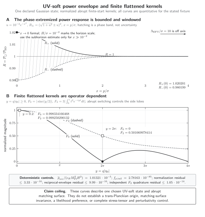
Bounded responses of the declared UV-soft benchmark. Panel A gives the exact phase extrema for $b=10^{-2}$; the hatched band collapses exponentially toward $R=1$, while $\Lambda_{\mathrm{EFT}}=10\sigma$ lies beyond the displayed signal window. Panel B compares two abruptly initialized, normalized time kernels. Both have a finite flattened value of one, but at $q|\eta_0|=2\pi$ the $I_0$ kernel vanishes while the $J_2$ kernel is approximately $0.50107$. The curves are quantitative for the stated equations and matching rule; they are not evidence for a trans-Planckian origin.

Open the full-size SVG, download the plotted CSV data, or inspect the complete semantic record.

The calculation therefore establishes a finite, operator-conditional signature, not a generic prediction of an excited state. Backreaction-compatible Gaussian states can leave squeezed signals too small to observe Flauger, Green, and Porto 2013, §§ 3.2 and 5.2.1, equations (5.2)–(5.3), Open PDF, while an independent cubic boundary kernel can produce a bispectrum even when the Gaussian power correction is small Agarwal et al. 2013, § 5.2, equations (5.30)–(5.32), Open PDF.

Boundary EFT, state regularity, and the matching surface

On a closed time contour, a general initial state may be written schematically as

$$\rho_0[\zeta^+,\zeta^-] = \mathcal N \exp\left\{ iS_0[\zeta^+,\zeta^-] \right\}, \qquad S_0=S_0^{(2)}+S_0^{(3)}+\cdots.$$

The quadratic kernel determines $N_k$ and $C_k$; $S_0^{(3)}$ determines intrinsic initial non-Gaussianity. A controlled calculation requires all of the following:

• $\rho_0$ is normalized, Hermitian, and positive.
• The relevant physical momenta satisfy $H\ll p$ where a subhorizon expansion is used and remain below the EFT and strong-coupling cutoffs. For a cubic correlator, the conservative boundary expansion also monitors $K/(a_0\Lambda_{\mathrm{EFT}})$.
• The state has the required short-distance regularity. Finite adiabatic order, full Hadamard behavior, and a chosen smooth cutoff are related checks, not synonyms.
• Bulk and initial-surface divergences are removed with the counterterms allowed by the same EFT.
• The renormalized stress, pressure, and their time dependence preserve the background, and loop and higher-kernel corrections remain perturbative.

Moving the surface is a test only if the same physical state is evolved and rematched. For the benchmark parameterization

$$\beta_k = \gamma_k e^{2ik\eta_0}, \qquad \gamma_k = be^{-(p/\sigma)^2}e^{i\vartheta},$$

a free-theory shift $\eta_0\to\eta_0+\Delta\eta$ that holds $\beta_k$ fixed requires

$$\gamma_k \longrightarrow \gamma_k e^{-2ik\Delta\eta}.$$

This formula treats $\gamma_k$ as an arbitrary function of comoving $k$. If the rematched state is rewritten in the same physical-width form on $a_1=a(\eta_0+\Delta\eta)$, it also requires

$$a_1\sigma_1=a_0\sigma_0, \qquad \sigma_1=\frac{a_0}{a_1}\sigma_0, \qquad \vartheta_1(k)=\vartheta-2k\Delta\eta.$$

The final phase is generally $k$ dependent, so the same state leaves the original one-parameter family with constant $\vartheta$. Changing $\eta_0$ while leaving $\gamma_k$, $\sigma$, or the constant phase untouched prepares a different state. With interactions, every quadratic, cubic, and counterterm kernel must be evolved to the new surface. The rematched correlators should then agree up to declared residuals such as

$$O\left[\left(\frac{p}{\Lambda_{\mathrm{EFT}}}\right)^{N+1}\right], \quad O\left(\frac{H}{p}\right), \quad O(\text{slow roll}), \quad O(\text{loops}).$$

The distinction is developed in Moving the Initial Surface.

A fixed $\eta_0$ is also different from a mode-dependent new-physics hypersurface such as $\eta_0(k)=-\Lambda/(Hk)$. The latter produces a prescription-dependent modulation in a particular matching model Danielsson 2002, § 2.3, equations 30–32, Open PDF; it is not a universal prediction of ultraviolet physics. Conversely, tracing a late mode to a trans-Planckian physical momentum does not by itself invalidate a low-energy prediction: sensitivity requires nonadiabatic evolution or state data that survive into the controlled regime Burgess, de Alwis, and Quevedo 2021, pp. 2–7, Open PDF.

What low-energy correlators can identify

Several very different constructions can end at the same low-energy state data. This table is wider than the text column; use horizontal scrolling, or focus it and press Left/Right, Home, or End.

From proposed origin to controlled low-energy data

Proposed origin	Required matching output	What a correlator can test	What it cannot establish alone
Quantum-cosmology saddle or contour	A normalized perturbative wavefunctional, its contour prescription, and quadratic and higher kernels	Whether those kernels give a controlled spectrum and bispectrum	That the saddle or contour is uniquely selected
Bounce or pre-inflationary evolution	A transfer map through the transition, including excited and non-Gaussian components	Correlated phases, windows, and shapes within the valid momentum band	That singularity resolution, rather than ordinary transient dynamics, caused them
Boundary EFT	Renormalized boundary coefficients, cutoff, truncation order, and positivity conditions	Power counting, regulator stability, and consistency among correlators	A unique ultraviolet completion of those coefficients
Mode-dependent matching prescription	The hypersurface rule, canonical variable, adiabatic order, and matching conditions	Predictions of that stated prescription	A model-independent trans-Planckian signal

Relative to the same reference modes and phase convention, equal $\alpha_k$ and $\beta_k$ fix the same zero-mean pure Gaussian state and hence all of its free Wick correlators. They do not fix independent non-Gaussian boundary kernels or bulk dynamics. Matching the retained Gaussian and non-Gaussian kernels, background, interaction Hamiltonian, cutoff prescription, and renormalization data is sufficient to guarantee the same power spectrum and bispectrum through that order; it is not necessary, because distinct effective data can yield the same selected observables through cancellations or other degeneracies.

Ordinary inflationary physics adds further alternatives: a sharp feature, resonant interaction, turn in field space, non-attractor phase, or pre-inflationary transient can imitate an oscillation or a flattened shape. A credible origin claim therefore needs correlated power-spectrum and bispectrum phases, EFT-compatible amplitudes, backreaction control, and robustness under conventional feature and foreground models. The broader inference workflow appears in Adversarial Control: Conventional Features and Foregrounds.

Executed controls and open gates

The benchmark must record negative results as carefully as passes. The table below distinguishes analytic variations that were actually carried out from tests that require a renormalized stress calculation or a likelihood pipeline and therefore remain open. It is wider than the text column; use horizontal scrolling, or focus it and press Left/Right, Home, or End.

Benchmark variations, residuals, and surviving claims

Control	Variation and fixed data	Recorded result	Status and claim ceiling
Matching surface	Shift η0 by any Δη inside the shared free-theory overlap while rematching γk and aσ so that βk is fixed	supk|Rnew − Rold| = 0 analytically	Pass for the free power spectrum. The isolated bispectrum term is not surface invariant until the induced cubic kernel and counterterms are evolved too.
Cutoff placement	Vary ΛEFT/σ through 8, 10, and 12 while holding the analytic Gaussian and the displayed band 0 ≤ p/σ ≤ 4 fixed	Rk is unchanged; fρ,tail = 3.31815 × 10−54, 2.78163 × 10−85, and 2.42151 × 10−123	Pass for cutoff placement in the declared Gaussian completion. The smooth profile itself was not varied, so regulator-profile robustness and arbitrary continuations remain open.
Adiabatic subtraction	Required variation: compare admissible state preparations of successive adiabatic order while applying complete fourth-order stress-tensor subtraction, or an equivalent covariant scheme, with the same renormalization conditions and initial-surface counterterms	No full instantaneous ⟨Tμν⟩ calculation was executed; a residual norm is therefore unavailable	Open. Retain only the finite diagonal occupation-energy screen, not a backreaction-safe claim.
Nuisance cosmology	Required variation: slow-roll transfer functions, ordinary features, foregrounds, calibration, covariance, and look-elsewhere range in one fixed likelihood	No likelihood fit was executed; significance and phase-coherence residuals are unavailable	Open. The fixture is an analytic response, not an anomaly, detection, or origin discriminator.

The surviving result is therefore deliberately narrow: the state has a reproducible power response, a finite conditional $\dot\zeta^3$ bispectrum contribution, an exact free surface-rematching check, and a negligible tail for the declared analytic completion. It has not passed full stress-tensor or nuisance-cosmology robustness. A future numerical analysis should add its resolution, covariance model, residual norm, and failure hypothesis to the same record.

What observations currently say

As of 30 August 2026, official Planck power-spectrum and excited-state bispectrum searches report no statistically significant signal. In the Planck non-Gaussianity conventions, the SMICA temperature-plus-polarization estimates were $60\pm43$ for the flattened template and $60\pm54$ for a generic non-Bunch–Davies template. An oscillatory non-Bunch–Davies template gave $-496\pm247$, about two standard deviations before a frequency-scan look-elsewhere correction that the collaboration noted would reduce its significance Planck 2018 Results IX (2020), § 5.2.7 and Table 12. The companion power-spectrum analysis found no significant nonparametric or joint power–bispectrum feature Planck 2018 Results X (2020), §§ 6–8 and 11.

Newer analyses constrain selected generic oscillatory power-spectrum amplitudes at roughly two to three percent at 95% confidence. Peng and Piao find $A_{\log}<0.0286$ and $A_{\mathrm{lin}}<0.0267$ using Planck, ACT DR6, and SPT-3G D1, with no significant preference in the tested templates Peng and Piao 2025, abstract and Tables II–III. Nerval et al. obtain $A_{\mathrm{lin}}<0.021$, $A_{\log}<0.022$, and $A_{\log\text{-}\mathrm{rf}}<0.023$ using Planck, ACT DR6, and DESI DR2; their Bayes factors moderately prefer the featureless reference model for the general-oscillation templates they test Nerval et al. 2026, § 5.1, Table 2, and § 5.3. A 2026 free-form reconstruction using Planck, ACT DR6, and SPT-3G D1 likewise reports no significant departure from a power law; its ACT small-scale blueward preference is about one standard deviation Chandra et al. 2026, abstract. All three are preprints at this page’s evidence cutoff, and none maps model-independently to $\beta_k$ or a non-Bunch–Davies state.

Current claim ceiling. Excited-state and oscillatory signals remain allowed but constrained, template dependent, and undetected. Even a future detection would first establish a correlated departure from featureless reference correlators, not a departure from the Bunch–Davies state or evidence for trans-Planckian physics. Identifying an initial-state effect, much less a particular quantum-cosmology program, would require the matching, conventional-dynamics, degeneracy, and robustness tests above.

Common pitfalls

Treating the interference sign as invariant. The sign changes when the phase of the reference mode changes. State the late-time phase convention and compare the invariant modulus.

Calling a rolloff scale a hard cutoff. A Gaussian is nonzero at every momentum. Separate its width from the EFT cutoff and report the energy-weighted tail.

Equating finite occupation energy with an admissible state. The diagonal $|\beta_k|^2$ integral is only one check. Positivity, Hadamard or adiabatic regularity, boundary renormalization, instantaneous stress, and perturbativity remain independent requirements.

Moving $\eta_0$ without rematching the state. This prepares a new state and can manufacture phase dependence. Evolve all retained kernels before testing surface independence.

Using $\alpha_k,\beta_k$ as complete initial-state data. Relative to a fixed reference basis, they completely specify a zero-mean pure Gaussian state. They do not specify a mixed state or independent non-Gaussian initial kernels.

Calling an oscillation trans-Planckian evidence. The same morphology can arise from controlled low-energy dynamics. Attribute an ultraviolet origin only after alternatives and matched-kernel degeneracies have been excluded.

Exercises

1. Exact power and phase convention

In the formal envelope limit $p/\sigma\to0$, take $b=0.1$ and $\alpha=\sqrt{1+b^2}$. Compute $R_k$ at an oscillation crest and trough. Then set $\alpha=1$ while keeping $\beta=0.1$ and identify which condition fails.

Solution to the exact-power exercise

At a crest and trough,

$$R_{\max}=(\alpha+b)^2, \qquad R_{\min}=(\alpha-b)^2.$$

With $\alpha=\sqrt{1.01}=1.00498756211209$,

$$R_{\max}=1.22099751242242, \qquad R_{\min}=0.819002487577582.$$

The linear approximation gives $1\pm0.2$ and misses the order-$b^2$ occupation and normalization terms. If $\alpha=1$, then

$$|\alpha|^2-|\beta|^2=0.99\ne1,$$

so the canonical Wronskian normalization fails even though one could still insert the numbers into a power-spectrum formula.

2. Energy, tail, and UV falloff

Evaluate $\overline{\rho}_{\mathrm{occ}}$ for the Gaussian benchmark and derive $f_{\rho,\mathrm{tail}}$. Check the numerical fixture. If instead $\beta(p)\sim p^{-q}$ at large $p$, for which $q$ is the diagonal occupation energy finite?

Solution to the energy-and-tail exercise

Spherical integration gives

$$\overline{\rho}_{\mathrm{occ}} = \frac{b^2}{2\pi^2} \int_0^\infty dp\,p^3e^{-2p^2/\sigma^2} = \frac{b^2\sigma^4}{16\pi^2}.$$

The same antiderivative above $p=\Lambda_{\mathrm{EFT}}$ gives

$$f_{\rho,\mathrm{tail}} = \left( 1+\frac{2\Lambda_{\mathrm{EFT}}^2}{\sigma^2} \right) e^{-2\Lambda_{\mathrm{EFT}}^2/\sigma^2}.$$

For $H=4\times10^{-5}M_{\mathrm{Pl}}$, $\sigma=100H$, $\Lambda_{\mathrm{EFT}}=10\sigma$, $b=10^{-2}$, and $\epsilon_H=10^{-2}$,

$$\overline{\rho}_{\mathrm{occ}} = 1.62114\times10^{-16}M_{\mathrm{Pl}}^4,$$ $$\frac{\overline{\rho}_{\mathrm{occ}}} {\epsilon_HM_{\mathrm{Pl}}^2H^2} = 1.01321\times10^{-5}, \qquad f_{\rho,\mathrm{tail}} = 2.78163\times10^{-85}.$$

For a power-law tail, the energy integrand scales as $p^{3-2q}$. Convergence requires $3-2q<-1$, or $q>2$. That is necessary for this diagonal integral but is not sufficient for full Hadamard regularity.

3. The regulated flattened limit

Use the same leading quasi-de Sitter initial slice as the cubic fixture, $\eta_0=-1/(a_0H)$, and take $q=0.2a_0H=2\times10^{-4}a_0\Lambda_{\mathrm{EFT}}$. Evaluate $|I_0(q)|$ and compare it with $I_0(0)$. Estimate the comoving width of the flattened enhancement. Then evaluate $J_2(0)$ and reproduce the phase envelope of the direct flattened $\dot\zeta^3$ insertion for the triangle and parameters used above.

Solution to the flattened-limit exercise

Using

$$|I_0(q)| = \frac{2|\sin(q\eta_0/2)|}{|q|},$$

and $q\eta_0=-0.2$ gives

$$|I_0| = \frac{2\sin(0.1)}{0.2a_0H} = \frac{0.998334166468}{a_0H}.$$

The exact flattened value is

$$I_0(0)=-\eta_0=\frac{1}{a_0H}.$$

The peak changes appreciably when $|q\eta_0|$ becomes order one, so its characteristic comoving width is $|q|\sim|\eta_0|^{-1}=a_0H=10^{-3}a_0\Lambda_{\mathrm{EFT}}$. The corresponding physical width on the initial slice is $H$. The finite initialization time regulates the apparent folded pole.

For the operator-specific kernel,

$$J_2(0) = \int_{\eta_0}^{0}\eta^2\,d\eta = \frac{(-\eta_0)^3}{3}.$$

At $p_1=\sigma$, $p_2=p_3=\sigma/2$, $\sigma/H=100$, and $|\beta_{k_1}|=be^{-1}$, the phase envelope is

$$\frac{\lambda_3}{24} \frac{p_1p_2p_3}{H^3} |\beta_{k_1}| = \frac{10^{-3}}{24} \frac{100^3}{4} \left(10^{-2}e^{-1}\right) =0.0383207751.$$

The $I_0$ and $J_2$ limits are both finite, but their momentum profiles differ because the cubic operator supplies different powers of conformal time.

4. A genuine surface-shift test

Suppose $\beta_k=\gamma_ke^{2ik\eta_0}$ describes a fixed free Gaussian state. Move the surface by $\Delta\eta$. How must $\gamma_k$ change if the physical state is to remain fixed? If it is rewritten with the same physical-width ansatz, how must $\sigma$ change? What mistake is made by holding these parameters fixed?

Solution to the surface-shift exercise

Requiring

$$\gamma_k'e^{2ik(\eta_0+\Delta\eta)} = \gamma_ke^{2ik\eta_0}$$

gives

$$\gamma_k' = \gamma_ke^{-2ik\Delta\eta}.$$

Holding $\gamma_k$ fixed instead changes the phase of $\beta_k$ and therefore changes the preparation. In an interacting theory this phase adjustment is only the quadratic part of the rematching; cubic kernels and boundary counterterms must evolve as well.

Writing the old envelope as $\exp[-k^2/(a_0^2\sigma_0^2)]$ and the new one as $\exp[-k^2/(a_1^2\sigma_1^2)]$ requires

$$a_1\sigma_1=a_0\sigma_0, \qquad \sigma_1=\frac{a_0}{a_1}\sigma_0.$$

The phase parameter becomes $\vartheta_1(k)=\vartheta-2k\Delta\eta$. Thus holding a constant $\vartheta$ and a fixed physical width $\sigma$ also prepares a different state.

5. Power-spectrum degeneracy in a mixed state

Construct a UV-soft nonvacuum Gaussian state with the same late-time power as the Bunch–Davies state. Verify positivity and explain why the two states are still physically different.

Solution to the mixed-state exercise

At each momentum choose

$$N_k = N_0e^{-2(p/\sigma)^2}, \qquad C_k=-N_k, \qquad N_0=0.01.$$

Then

$$1+2N_k+2\operatorname{Re}C_k=1,$$

so the late-time power equals the Bunch–Davies value. Positivity holds mode by mode because

$$|C_k|^2=N_k^2 \le N_k(N_k+1).$$

The Gaussian falloff makes the diagonal occupation-energy integral UV finite. The constructed state is Gaussian, so its intrinsic connected cubic kernel vanishes. It is nevertheless physically different because its unequal-time covariance and stress tensor differ, and a nonzero bulk interaction generally produces a different bispectrum. If non-Gaussian states are admitted, an independently matched cubic boundary kernel supplies an additional degeneracy. One equal two-point observable therefore does not identify the state.

The complete semiclassical-status assessment continues with Semiclassical Recovery, Decoherence, Obstructions, and Status. For mutable source updates, open problems, and entry points to current work, continue to the Holography and Quantum Gravity research guide.

Use the chapter structure diagram to place this initial-state handoff among the chapter’s routes, and the validity and failure diagram to identify where a state, observable, or singularity-resolution claim can fail.

For the chapter-wide comparison of assumptions, counterevidence, falsifiers, and claim ceilings, see the claim-domain table.

References

• Agarwal, N., R. Holman, A. J. Tolley, and J. Lin. “Effective Field Theory and Non-Gaussianity from General Inflationary States.” Journal of High Energy Physics 2013, 5 (2013): 085. DOI. Open PDF.
• Burgess, C. P., S. P. de Alwis, and F. Quevedo. “Cosmological Trans-Planckian Conjectures Are Not Effective.” Journal of Cosmology and Astroparticle Physics 2021, 5 (2021): 037. DOI. Open PDF.
• Chandra, D., D. K. Hazra, A. Shafieloo, and T. Souradeep. “The Primordial Power Spectrum from the Largest to Smallest CMB Scales.” arXiv:2608.24413 (2026), preprint. Preprint.
• Collins, H., and R. Holman. “Renormalization of Initial Conditions and the Trans-Planckian Problem of Inflation.” Physical Review D 71 (2005): 085009. DOI. Open PDF.
• Collins, H., and R. Holman. “The Renormalization of the Energy-Momentum Tensor for an Effective Initial State.” Physical Review D 74 (2006): 045009. DOI. Open PDF.
• Danielsson, U. H. “A Note on Inflation and Trans-Planckian Physics.” Physical Review D 66 (2002): 023511. DOI. Open PDF.
• Flauger, R., D. Green, and R. A. Porto. “On Squeezed Limits in Single-Field Inflation. Part I.” Journal of Cosmology and Astroparticle Physics 2013, 8 (2013): 032. DOI. Open PDF.
• Holman, R., and A. J. Tolley. “Enhanced Non-Gaussianity from Excited Initial States.” Journal of Cosmology and Astroparticle Physics 2008, 5 (2008): 001. DOI. Open PDF.
• Junker, W., and E. Schrohe. “Adiabatic Vacuum States on General Spacetime Manifolds: Definition, Construction, and Physical Properties.” Annales Henri Poincaré 3, 6 (2002): 1113–1181. DOI. Open PDF.
• Meerburg, P. D., J. P. van der Schaar, and P. S. Corasaniti. “Signatures of Initial State Modifications on Bispectrum Statistics.” Journal of Cosmology and Astroparticle Physics 2009, 5 (2009): 018. DOI. Open PDF.
• Nerval, S. K., R. Hlozek, H. T. Jense, and J. R. Bond. “Constraining Primordial Oscillations and Inflationary Particle Production with Planck, ACT DR6, and DESI DR2.” arXiv:2606.28310 (2026), preprint. Preprint.
• Peng, Z.-Y., and Y.-S. Piao. “Tightening Constraints on Primordial Oscillations with Latest ACT and SPT Data.” arXiv:2507.17276v2 (2025), preprint. Preprint.
• Planck Collaboration. “Planck 2018 Results. IX. Constraints on Primordial Non-Gaussianity.” Astronomy & Astrophysics 641 (2020): A9. DOI. Open PDF.
• Planck Collaboration. “Planck 2018 Results. X. Constraints on Inflation.” Astronomy & Astrophysics 641 (2020): A10. DOI. Open PDF.