Lorentzian, Nonequilibrium, and Chaotic Holography

Lorentzian holography maps a boundary real-time observable to a bulk problem only after the contour, initial state, operator ordering, source, horizon or interior condition, response channel, and observation window are fixed. This chapter develops that map from retarded correlators through nonequilibrium geometry and chaos, then shows why a classical horizon cannot determine exact finite-$N$ late time.

Helpful background. Closed-Time-Path Generating Functionals in Practice supplies real-time contours; Out-of-Time-Order Correlators and Contour Regularization supplies OTOCs; Hydrodynamic Attractors and Asymptotic Gradient Expansions supplies attractors; AdS Black Branes and Holographic Thermodynamics supplies the equilibrium saddle.

The data that define a real-time observable

Before solving a bulk equation, state:

1. the density matrix or Euclidean preparation and every contour segment;
2. the operator ordering and Fourier convention;
3. the source, response coefficient, and counterterm scheme;
4. the future-horizon, past-horizon, cap, or horizonless interior condition;
5. the gauge-invariant fluctuation channel;
6. the large-$N$, coupling, frequency, momentum, and time limits;
7. the first correction that can defeat the classical saddle.

The response route begins with items 1–5 and proceeds from an infalling solution to poles or open-system kernels. The dynamics route begins with a prepared time-dependent state and compares multiple boundary probes before discussing hydrodynamization, shockwaves, or late-time spectra.

Check your preparation

You are ready to enter if you can distinguish retarded, advanced, time-ordered, and regulated OTO correlators; explain why a thermal state uses a Euclidean segment; and distinguish event from apparent horizons.

• For response functions, use the first helpful-background link and begin with pages 1–6.
• For far-from-equilibrium evolution, begin with pages 2–3, then 7–9.
• For chaos or late time, read the OTOC background before pages 10–12.

Knowing a Euclidean correlator does not by itself determine a Lorentzian ordering, and knowing a classical metric does not determine the exact state.

Choose a route

Goal	Route through the numbered guide	Required stopping test
Compute linear response	1–2, then 5–6	Is the contour, source/response normalization, and invariant channel fixed?
Prepare and evolve a state	2–3, then 7–9	Do all claimed probes equilibrate within the stated tolerance?
Derive noise or dissipation	2 and 4	Do KMS, positivity, causality, and memory-scale checks pass?
Analyze scrambling	1, 10–12	Is the regulator and elastic large-$N$ window explicit?
Diagnose an overclaim	11–12	Was a saddle result extended to a different horizon or exact finite $N$?

Chapter guide

1. Lorentzian Holographic Correlators and Infalling Conditions derives the source–response ratio and spectral flux for a retarded black-brane correlator.
2. Schwinger–Keldysh Contours and Real-Time Bulk Geometries glues Euclidean and doubled Lorentzian saddles and tests normalization and KMS.
3. Holographic Initial States and Euclidean Caps converts cap sources into normalizable Lorentzian initial data and rejects singular preparations.
4. Holographic Influence Functionals and Open-Sector Dynamics extracts causal dissipation and symmetrized noise before testing the Markovian limit.
5. Quasinormal Modes, Poles, and Spectral Response solves the infalling, source-free eigenproblem and separates poles from finite-$N$ levels.
6. Bulk Quasinormal Modes and Boundary Hydrodynamic Poles derives shear, sound, and diffusion dispersions in invariant channels.
7. Time-Dependent Geometries and Holographic Thermalization compares local, geodesic, and extremal-surface probes in collapse.
8. Holographic Quenches and Entanglement Growth extracts growth and saturation while bounding entanglement-velocity claims.
9. Holographic Hydrodynamization, Attractors, and Gradient Asymptotics separates asymptotic hydrodynamics from quasinormal transients and initial-state dependence.
10. Shockwaves, OTOCs, and Scrambling derives the eikonal growth, butterfly front, and scrambling window for a regulated OTOC.
11. Real-Time Claims, Horizons, and Validity Limits identifies which response statements survive changes of horizon type or time regime.
12. Finite-N Spectra, Recurrences, and the Late-Time Plateau compares smooth saddle decay with discrete spectra, averaged ramps, plateaus, and recurrences.

One hierarchy, several physical claims

The central sequence is

$$\text{contour and state} \longrightarrow \text{causal bulk boundary problem} \longrightarrow \text{retarded poles or time-dependent saddle} \longrightarrow \text{bounded real-time conclusion}.$$

Infalling conditions yield retarded response in the declared thermal state Son and Starinets 2002. Glued contour saddles yield all Schwinger–Keldysh components consistently Skenderis and van Rees 2009. Shockwaves give leading OTOC growth before scrambling Shenker and Stanford 2014. At finite $N$, discrete spectral sums replace exact irreversible decay; averaged random-matrix behavior is a further, observable-specific statement Cotler et al. 2017.

These results are complementary, not interchangeable. A quasinormal pole is not a microscopic energy level; an apparent horizon is not an observable-independent thermalization time; OTOC growth is not a complete spectral-chaos diagnosis; and a plateau after averaging is not automatically a fixed-theory unitarity calculation.

Review the chapter

Causal prescription. Starting from a scalar near a future horizon, derive the infalling exponent and $G_R\propto B/A$. A successful answer identifies the contour, Fourier sign, flux direction, and contact ambiguity.

Contour consistency. Glue a thermal two-leg saddle. The answer must state field and oriented-momentum matching, recover $Z[J,J]=1$, and verify KMS.

Pole matching. Derive $\omega=-i\eta k^2/(\epsilon+p)$ in the shear channel. The answer must use a gauge-invariant field and distinguish a pole from a frame-dependent coefficient.

Probe dependence. Compare one local and two nonlocal probes in collapse. A complete answer explains why apparent-horizon formation cannot be their common equilibration time.

Chaos window. Derive $t_*\sim(\beta/2\pi)\log N^2$. The answer must name the regulator, eikonal approximation, spatial channel, and failure at order-one OTOC correction.

Late time. Estimate $t_H$ from the mean level spacing. The answer must distinguish fixed-theory, time-averaged, and disorder-averaged observables and reject exact exponential decay at finite $N$.

Continue from here

Proceed to Holographic Matter, Transport, and Model Building to apply retarded and hydrodynamic methods at finite density. Return to Thermal and Nonequilibrium QFT for the general contour, response, hydrodynamic, and chaos theory, or to the volume overview for black-hole information and entropy routes.

Evidence cutoff: 25 July 2026. Current-sensitive interpretations are fixed to this date. No classical-saddle result is used here as an exact finite-$N$ completion.

Chapter-scale structure and validity checks

The chapter-scale structure map locates this page’s result inside the full reasoning chain. Follow the solid arrows through the declared inputs and checks; the dashed final arrow marks the point where an additional inference would be required.

Real-time holography depends on contour, state preparation, causal boundary conditions, and a declared time window; horizons do not fix exact late time. The diagram is an original schematic, is not to scale, and uses the dashed final arrow to mark the claim boundary.

Accessible figure data (JSON)

The companion validity map turns three common overclaims into explicit failure tests. Read each row from its declared object to the diagnostic, then compare the licensed conclusion with the dashed “not” endpoint.

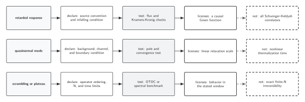
Real-time holography depends on contour, state preparation, causal boundary conditions, and a declared time window; horizons do not fix exact late time. Each row pairs a diagnostic with the strongest supported conclusion and an explicitly unsupported promotion. The diagram is an original schematic and is not to scale.

Accessible figure data (JSON)

Claim-domain comparison

The table below gives a screen-reader-friendly comparison of three representative claims. It keeps the required declaration, approximation status, evidence timing, counterevidence, falsifier, failure condition, and licensed conclusion in one reading order.

Representative claim domains and validity boundaries for Lorentzian, Nonequilibrium, and Chaotic Holography

Claim object	State, ensemble, and conventions	Approximation, status, and evidence timing	Uncertainty and counterevidence	Falsifier	Failure condition	Licensed conclusion
retarded response	Declare source convention and infalling condition; use the volume conventions unless the page states a local replacement.	Model-specific calculation or conditional result. Control chain: real-time contour and state → Lorentzian bulk geometry → initial and horizon conditions → poles, response, and chaos tests → time-window conclusion. Sources are cited on the destination page; literature checked through 10 August 2026.	Track omitted corrections, alternate branches, and competing definitions. A failed “flux and Kramers-Kronig checks” check is counterevidence to the promoted claim.	flux and Kramers-Kronig checks	all Schwinger-Keldysh correlators	a causal Green function
quasinormal mode	Declare background, channel, and boundary condition; use the volume conventions unless the page states a local replacement.	Model-specific calculation or conditional result. Control chain: real-time contour and state → Lorentzian bulk geometry → initial and horizon conditions → poles, response, and chaos tests → time-window conclusion. Sources are cited on the destination page; literature checked through 10 August 2026.	Track omitted corrections, alternate branches, and competing definitions. A failed “pole and convergence test” check is counterevidence to the promoted claim.	pole and convergence test	nonlinear thermalization time	linear relaxation scale
scrambling or plateau	Declare operator ordering, N, and time limits; use the volume conventions unless the page states a local replacement.	Model-specific calculation or conditional result. Control chain: real-time contour and state → Lorentzian bulk geometry → initial and horizon conditions → poles, response, and chaos tests → time-window conclusion. Sources are cited on the destination page; literature checked through 10 August 2026.	Track omitted corrections, alternate branches, and competing definitions. A failed “OTOC or spectral benchmark” check is counterevidence to the promoted claim.	OTOC or spectral benchmark	exact finite-N irreversibility	behavior in the stated window

Download the structured table data (JSON).

References

• Cotler, Jordan S.; Gur-Ari, Guy; Hanada, Masanori; Polchinski, Joseph; Saad, Phil; Shenker, Stephen H.; Stanford, Douglas; Streicher, Alexandre; and Tezuka, Masaki. “Black Holes and Random Matrices.” Journal of High Energy Physics 2017, 118 (2017). doi:10.1007/JHEP05(2017)118.
• Shenker, Stephen H., and Douglas Stanford. “Black Holes and the Butterfly Effect.” Journal of High Energy Physics 2014, 067 (2014). doi:10.1007/JHEP03(2014)067.
• Skenderis, Kostas, and Balt C. van Rees. “Real-Time Gauge/Gravity Duality: Prescription, Renormalization and Examples.” Journal of High Energy Physics 2009, 085 (2009). doi:10.1088/1126-6708/2009/05/085.
• Son, Dam T., and Andrei O. Starinets. “Minkowski-Space Correlators in AdS/CFT Correspondence: Recipe and Applications.” Journal of High Energy Physics 2002, 042 (2002). doi:10.1088/1126-6708/2002/09/042.