Baby Universes, Alpha Parameters, and Proposed Superselection Sectors

Here a baby universe means a compact spatial component on a cut, with no selected asymptotic boundary. It need not be small, and it is not the same thing as a closed Euclidean vacuum component that merely multiplies a path-integral normalization. A Euclidean wormhole can propagate such data between mouths and, in a dilute approximation, induce a bilocal interaction in the parent universe. That interaction may admit an auxiliary alpha representation. The extra conclusion that alpha labels a physical state—or a superselection sector—requires a positive Hilbert-space construction, a complete enough observable algebra, and proof that allowed operations preserve its spectral projectors.

The logical order matters:

$$\text{wormhole pair} \Longrightarrow \text{bilocal kernel} \Longrightarrow \text{auxiliary }\alpha \quad\not\Longrightarrow\quad \text{physical }\alpha\text{ sector}.$$

The last implication needs new hypotheses. This page derives the earlier arrows, constructs a transparent parent–baby toy model, and then states the additional conditions under which the spectral language is justified. It does not infer that a single fixed boundary theory is an ensemble.

Required background. Euclidean Wormholes and Connected Boundary Amplitudes: what a connected term licenses supplies the gravitational amplitude and its contour-dependent coefficient. Fixed-Theory, Ensemble, and Superselection Claims: superselection relative to an algebra fixes the meanings of a fixed theory, a shared sector, and an ensemble average.

Helpful background. Superselection Rules and Accessible Entanglement develops the operational algebraic language. Replica Wormholes and Saddle Competition is a nearby topology-changing calculation with a different observable.

Evidence cutoff. 29 August 2026. The Hilbert-space interpretation and one-dimensionality claims below remain conditional research statements, not settled consequences of the semiclassical wormhole expansion.

Baby-universe states on a cut

Cut a Euclidean history across a compact spatial slice. Boundary preparations on one side define formal vectors, and gluing a preparation to the reflected preparation defines their pairing. A physical baby-universe Hilbert space exists only if this pairing is positive semidefinite. One must then quotient every zero-norm vector and complete the quotient. In symbols,

$$\mathcal V_{\rm prep} \xrightarrow{\ \langle\cdot,\cdot\rangle_{\rm PI}\ge 0\ } \mathcal V_{\rm prep}/\mathcal N \xrightarrow{\ \text{completion}\ } \mathcal H_{\rm BU}, \qquad \mathcal N=\{v:\langle v,v\rangle_{\rm PI}=0\}.$$

This distinction is easy to miss. A third-quantized Fock space can be useful in a dilute semiclassical expansion,

$$\mathcal H_{\rm kin} \simeq \mathcal H_P\otimes\mathcal F(\mathcal H_{1{\rm BU}}),$$

but nonperturbative relations can turn apparently different kinematic configurations into the same physical state after the null quotient. The quotient, not the number of semiclassical drawings, determines the physical dimension. Marolf and Maxfield 2020, §§2.1–2.3, eqs. (5)–(19) give the path-integral construction and emphasize this distinction.

Let $\widehat Z[J]$ adjoin an asymptotic boundary with sources $J$. Permuting disjoint boundary insertions and reflecting their source data gives the formal relations

$$[\widehat Z[J],\widehat Z[J']]=0, \qquad \widehat Z[J]^\dagger=\widehat Z[J^*].$$

Closure under $J\mapsto J^*$ makes a bounded represented family normal. For unbounded representatives, pairwise commutators on a common domain are not enough: require strongly commuting spectral measures, or work with an appropriate bounded functional calculus. Under that stronger operator condition, the joint spectral theorem supplies labels $\alpha$ such that

$$\widehat Z[J]\lvert\alpha\rangle =Z_\alpha[J]\lvert\alpha\rangle.$$

For a normalizable Hartle–Hawking preparation, the normalized multi-boundary expectation value then has the spectral representation

$$\frac{ \langle{\rm HH}\rvert \prod_{a=1}^{m}\widehat Z[J_a] \lvert{\rm HH}\rangle }{ \langle{\rm HH}\vert{\rm HH}\rangle } = \int \mu_{\rm HH}(d\alpha) \prod_{a=1}^{m}Z_\alpha[J_a].$$

Continuous-spectrum symbols $\lvert\alpha\rangle$ are delta-normalized generalized eigenvectors. Operational conditioning should first use a finite spectral set $\Delta$ and its projector $P(\Delta)$, and only then take a controlled sharp-window limit. Marolf and Maxfield 2020, §§2.2–2.4, eqs. (10)–(29) develop this spectral construction.

A dilute wormhole gas produces a bilocal kernel

Choose a finite real basis of integrated parent-universe insertions,

$$\mathcal O_i = \int d^Dx\,\sqrt g\,O_i(x), \qquad i=1,\ldots,N.$$

Suppose one small wormhole contributes $\tfrac12 C_{ij}\mathcal O_i\mathcal O_j$. If wormholes are dilute, mutually noninteracting, and summed with the usual $1/m!$ combinatorics, then

$$\sum_{m=0}^{\infty} \frac1{m!} \left(\frac12 C_{ij}\mathcal O_i\mathcal O_j\right)^m = \exp\!\left(\frac12 C_{ij}\mathcal O_i\mathcal O_j\right).$$

The matrix $C$ packages the admitted wormhole family, mouth amplitudes, moduli integration, and contour coefficient. This exponentiation is therefore conditional: interactions between wormholes, additional topologies, negative modes, or a vanishing thimble coefficient can change it. The preceding page owns those gravitational acceptance tests.

The classic topology-change and coupling-constant constructions are developed in Giddings and Strominger 1988, pp. 890–907, Giddings and Strominger 1989, pp. 481–508, and Coleman 1988, pp. 643–668. The derivation here states its finite-basis and contour assumptions explicitly because the historical interpretation is not automatic in a modern fixed-theory setting.

For real symmetric positive-definite $C$, define

$$p_C(\alpha) = \frac{ \exp[-\tfrac12\alpha^{\mathsf T}C^{-1}\alpha] }{ \sqrt{(2\pi)^N\det C} }.$$

Completing the square gives the normalized Hubbard–Stratonovich identity

$$\exp\!\left(\frac12C_{ij}\mathcal O_i\mathcal O_j\right) = \int_{\mathbb R^N}d^N\alpha\, p_C(\alpha) \exp(\alpha_i\mathcal O_i).$$

With the Euclidean convention

$$I_P(\lambda)=I_{\rm base}+\lambda_i\mathcal O_i,$$

the integrand $e^{-I_P(\lambda)}e^{\alpha_i\mathcal O_i}$ is the parent theory with

$$\lambda_i^{\rm eff}=\lambda_i-\alpha_i.$$

The sign is a consequence of this declared convention, not a universal mnemonic. Dimensional consistency requires

$$[\alpha_i\mathcal O_i]=[C_{ij}\mathcal O_i\mathcal O_j]=1.$$

If $C$ is indefinite, nonreal, or inherited from a complex gravitational contour, the same algebra may require a deformed integration cycle and a complex weight. It is then a contour representation, not a probability distribution.

A parent–baby toy model

The Gaussian identity can be represented as a genuine expectation value without pretending that this representation derives the gravitational Hilbert space. Take

$$\mathcal H_{\rm tot} = \mathcal H_P\otimes\mathcal H_{\rm BU}^{\rm toy}, \qquad \mathcal H_{\rm BU}^{\rm toy} = L^2(\mathbb R^N,d^N\alpha),$$

and let $\widehat\alpha_i$ act by multiplication,

$$(\widehat\alpha_i\psi)(\alpha)=\alpha_i\psi(\alpha).$$

Prepare $\psi_C(\alpha)=\sqrt{p_C(\alpha)}$. For commuting Euclidean c-number insertions,

$$\langle\psi_C\rvert e^{\widehat\alpha_i\mathcal O_i} \lvert\psi_C\rangle = \int d^N\alpha\,p_C(\alpha)e^{\alpha_i\mathcal O_i} = e^{\frac12C_{ij}\mathcal O_i\mathcal O_j}.$$

Thus the bilocal factor is exactly a moment-generating function in this toy model. The calculation does not prove that a gravitational path integral has the required positive inner product or that these multiplication operators exhaust its boundary algebra.

For real-time evolution, make further assumptions: every fiber uses a common parent Hilbert space and common dense domain, $\alpha\mapsto H_P(\lambda-\alpha)$ is a measurable self-adjoint decomposable family, and the Hamiltonian contains no alpha-mixing terms. Then

$$H_{\rm tot} = H_P(\lambda-\widehat\alpha) = \int_{\mathbb R^N}^{\oplus} d^N\alpha\,H_P(\lambda-\alpha), \qquad U(t)=\int^{\oplus}d^N\alpha\,U_\alpha(t).$$

Starting from $\rho_P\otimes\lvert\psi_C\rangle\langle\psi_C\rvert$ and tracing out the baby factor gives

$$\rho_P(t) = \int d^N\alpha\,p_C(\alpha) U_\alpha(t)\rho_PU_\alpha^\dagger(t).$$

This formula separates three statements that are often blurred together:

• A sharp $\alpha$ selects one unitary parent evolution with definite shifted couplings.
• A coherent baby state can entangle the parent and baby factors.
• Ignoring the baby factor produces a random-unitary channel for the parent.

None of the three establishes that a fixed boundary QFT has randomly drawn couplings. In particular, random-looking describes the reduced or unconditioned description; at sharp $\alpha$, the coupling is definite.

Shared alpha and the connected covariance

The distinction becomes quantitative with two boundaries. Let $Z_a(\alpha)$ be the one-boundary amplitude in a sharp sector and let $G_{12,c}^{(\alpha)}$ denote any connected contribution that remains inside that sector. The total connected amplitude is

$$G_{12}^{c} = \int\mu(d\alpha)\,G_{12,c}^{(\alpha)} + \operatorname{Cov}_{\mu} \!\left(Z_1(\alpha),Z_2(\alpha)\right).$$

The second term is the covariance of a shared alpha label. It is not the whole answer unless $G_{12,c}^{(\alpha)}=0$. Exact simultaneous eigenstates of the complete commuting boundary-insertion algebra have this factorization property for those insertions; a semiclassical Gaussian rewrite alone does not establish it.

For a reproducible one-parameter example, take

$$Z_a(\alpha)=z_a e^{\alpha j_a}, \qquad \alpha\sim\mathcal N(0,C), \qquad C>0.$$

The Gaussian moment-generating function gives

$$\overline{Z_a} =z_a e^{Cj_a^2/2}, \qquad \overline{Z_1Z_2} =z_1z_2e^{C(j_1+j_2)^2/2},$$

and hence

$$\operatorname{Cov}(Z_1,Z_2) = \overline{Z_1}\,\overline{Z_2} \left(e^{Cj_1j_2}-1\right).$$

Three checks expose the protocol. The covariance vanishes when $C\to0$ or either $j_a=0$. It also vanishes if the two boundaries receive independent redraws,

$$\int\mu(d\alpha_1)\mu(d\alpha_2) Z_1(\alpha_1)Z_2(\alpha_2) = \overline{Z_1}\,\overline{Z_2}.$$

Thus “average over alpha” is incomplete bookkeeping: one must say whether the label persists across the experiment, is independently redrawn, or is conditioned to a spectral window.

There is one more identification test. Let $\mathsf A_{\rm spec}$ be the joint spectrum of the physical boundary operators, and use $\beta\in\mathbb R^N$ for the Gaussian auxiliary variable. Naming both variables alpha does not make them the same. One sufficient matching contract is a measurable map

$$f:\mathsf A_{\rm spec}\longrightarrow\mathbb R^N, \qquad f_*\mu_{\rm HH}=p_C(\beta)\,d^N\beta,$$

together with the effective action

$$I_{\rm eff}(\xi) = I_{\rm base} +[\lambda_i-f_i(\xi)]\mathcal O_i, \qquad \xi\in\mathsf A_{\rm spec},$$

on the declared generating algebra. A unitary equivalence intertwining the corresponding cyclic representations is a stronger alternative. Positivity and the spectral theorem build the physical side; this pushforward-and-action match is what identifies it with the particular Gaussian rewrite.

The following diagram keeps the formal Gaussian rewrite and the physical spectral construction on separate tracks. Follow the dashed gate: it lists exactly what must be added before auxiliary alpha can be interpreted as sector data.

On a narrow screen, swipe or use the Left and Right arrow keys to pan across the figure. Home and End move to its edges. A full-size link is also available.

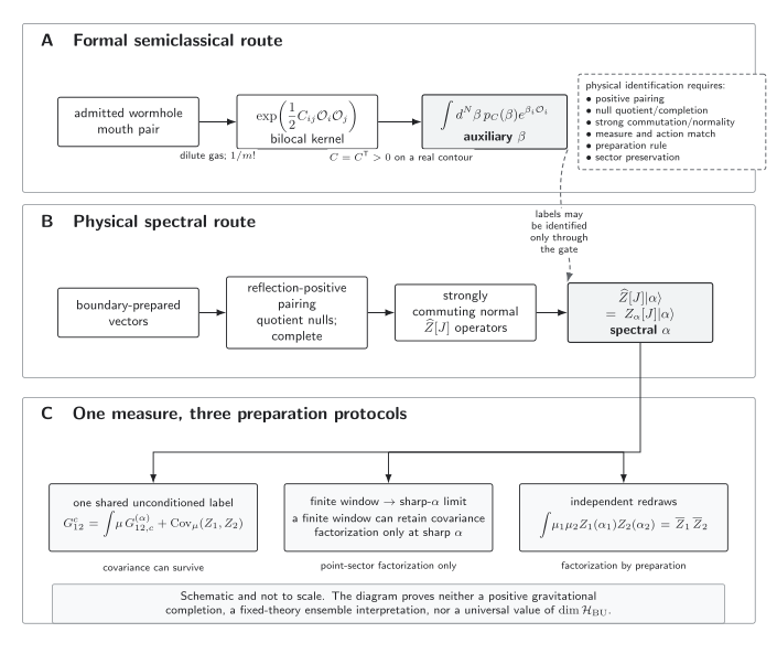
The Hubbard–Stratonovich route is an algebraic representation of a controlled bilocal kernel. The spectral route additionally constructs $\mathcal H_{\rm BU}$ and its strongly commuting normal boundary operators. Identifying their labels also requires the displayed measure-and-action match. A shared unconditioned label can produce covariance; a finite spectral window can retain it; only a controlled sharp-alpha limit factorizes the complete commuting insertion algebra. Independent redraws factorize for a different reason. Original schematic, not to scale; it does not prove that gravity supplies the gated hypotheses. Accessible figure data (JSON)

The figure has the following text-equivalent content.

Track or protocol	Defined object	Licensed conclusion	Missing or failed condition
Dilute wormhole track	$\exp(\tfrac12C_{ij}\mathcal O_i\mathcal O_j)$	A stated topology sum yields a bilocal kernel	Contour coefficient, interactions, and omitted topologies remain controlled inputs
Gaussian track	$\int d^N\beta\,p_C(\beta)e^{\beta_i\mathcal O_i}$	Positive $C$ gives an auxiliary-variable identity	No gravitational Hilbert space or superselection follows
Spectral track	$\widehat Z[J]\lvert\alpha\rangle=Z_\alpha[J]\lvert\alpha\rangle$	A positive null-quotiented and completed construction gives joint spectral labels for strongly commuting normal operators	It still needs an accessible algebra and sector preservation
Identification gate	$f_*\mu_{\rm HH}=p_C(\beta)d^N\beta$ and $I_{\rm eff}=I_{\rm base}+[\lambda_i-f_i(\alpha)]\mathcal O_i$	The spectral representation matches the declared Gaussian measure and coupling action	Positivity, a null quotient, and a shared symbol alone do not establish this match
One shared label	$\int\mu(d\alpha)Z_1(\alpha)Z_2(\alpha)$	Sector uncertainty can correlate boundaries	Residual fixed-alpha connectivity must be checked separately
Finite window to sharp limit	$P(\Delta)$, followed by a controlled point-sector limit	The complete commuting insertion algebra factorizes only at sharp $\alpha$	A finite window generally retains within-window covariance, and a larger algebra may contain intertwiners
Independent redraws	$\int\mu(d\alpha_1)\mu(d\alpha_2)Z_1(\alpha_1)Z_2(\alpha_2)$	The two sampled experiments factorize	This is a different preparation protocol, not conditioning

Superselection is an algebraic preservation statement

Let $P_{\widehat\alpha}(\Delta)$ be the joint spectral projector for a Borel set $\Delta$. Alpha is superselected relative to an accessible algebra $\mathcal A_{\rm acc}$ only if

$$[A,P_{\widehat\alpha}(\Delta)]=0 \qquad \text{for every }A\in\mathcal A_{\rm acc} \text{ and every }\Delta.$$

Using projectors rather than a formal commutator with an unbounded $\widehat\alpha$ avoids a domain ambiguity. It also makes the qualification “relative to an algebra” unavoidable. The full algebra $B(\mathcal H_P\otimes\mathcal H_{\rm BU})$ generally contains operators that move between fibers.

A two-sector laboratory makes the point. On $\mathcal H_{\rm BU}=\operatorname{span}\{\lvert+\rangle,\lvert-\rangle\}$, set

$$\widehat\alpha=a(\lvert+\rangle\langle+\rvert-\lvert-\rangle\langle-\rvert), \qquad \lvert\psi\rangle =c_+\lvert+\rangle+c_-e^{i\phi}\lvert-\rangle.$$

Every diagonal accessible observable is insensitive to the relative phase $\phi$. But the intertwiner

$$T=\lvert+\rangle\langle-\rvert+\lvert-\rangle\langle+\rvert$$

has $[T,\widehat\alpha]\ne0$ and detects that phase. If $T$ is allowed, the proposed sectors fail for the enlarged algebra. In the continuous toy model, a perturbation proportional to the conjugate momentum $\widehat\pi_i$ similarly moves alpha because $[\widehat\pi_j,\widehat\alpha_i]=-i\delta_{ij}$.

Four uses of the word alpha should therefore remain distinct.

Meaning	Mathematical role	Physical status
Hubbard–Stratonovich alpha	Integration variable for one kernel	Algebraic until a contour and measure are specified
Spectral alpha	Joint value of represented commuting boundary operators	Physical only after the positive Hilbert-space construction
Shared sector mixture	One persistent label with state $\mu$ on the accessible algebra	Operationally equivalent to any model inducing the same full state on that algebra
Ensemble member	A theory drawn from a distribution of theories	Requires a sampling interpretation not supplied by spectral decomposition alone

Higher moments do not automatically distinguish the last two rows. If the measure, persistent-label protocol, and accessible commuting algebra agree, then all their moments agree. A distinction requires independent redraws, conditioning access, coherent intertwiners, or some other observable or preparation rule outside that common description.

Comparing one-dimensionality claims with assumptions held fixed

Two influential arguments use “one-dimensional” for different constructions. Before comparing them, freeze the contract

$$\mathfrak C = (\text{completion},d,\mathcal H,\mathcal A_{\rm acc}, \text{null quotient},W,\text{entanglement},\text{measurement rule}).$$

Changing a field in $\mathfrak C$ changes the question. The following comparison therefore repeats the same fields rather than treating the papers as a simple claim and counterclaim.

Contract field	McNamara–Vafa	Antonini–Rath–Sasieta–Swingle–Vilar López
Completion and dimension	Complete unitary quantum gravity in spacetime dimension $d>3$, with possible low-dimensional exceptions discussed separately	A particular asymptotically AdS big-bang/big-crunch construction and its proposed CFT encoding
Hilbert space being counted	Exact gauge-invariant empty-boundary space $\mathcal H_{\rm QG}(\varnothing)$ after gauge and null identifications	Perturbative closed-universe code/domain and its image under an exterior encoding map $W$; these are not automatically the exact empty-boundary space
Main hypotheses	No free parameters, no global $(-1)$-form symmetry, cobordism-related reasoning, and standard non-ensemble AdS/CFT boundary locality	A postselected or non-isometric encoding whose distinguishability depends on exterior entanglement and on the chosen internal observable rule
Rank statement	The Baby Universe Hypothesis proposes $\dim\mathcal H_{\rm BU}=1$	At zero exterior entanglement the external Gram matrix is rank one; with sufficient entanglement the model’s $W$ can become approximately isometric on the declared code space
Claim ceiling	A swampland-motivated conjecture about the exact physical theory, not a theorem extracted from the dilute wormhole gas	A model-specific encoding proposal, not a universal theorem that the exact baby-universe Hilbert space is large

McNamara and Vafa’s arguments are therefore stronger and narrower than “completeness makes the space one-dimensional.” They combine the absence of free parameters—including discrete possibilities in their discussion—a proposed no-global-$(-1)$-form principle, cobordism input, and a separate boundary-locality argument in standard AdS/CFT. Their state–operator discussion targets strictly well-defined exact compactly supported bulk operators; it does not eliminate ordinary relational or code-subspace quasi-local observables. See McNamara and Vafa 2020, §§3.1–3.4 and §§4.1–4.3.

Antonini and collaborators instead distinguish a large perturbative closed-universe description from what an exterior CFT encoding can distinguish. In their tensor-network notation, $\mathsf M$ is the closed-universe input space and $\mathsf{lr}$ is the entangled AdS-side resource mapped toward the exterior CFT. A model-dependent full-space approximate-isometry condition then requires $S(\mathsf{lr})>2S(\mathsf M)$. At zero entanglement the external image becomes rank one. They retain a rich effective internal description through postselection or a coarse-grained observer rule, but the associated final-state proposal leaves global causality, unitarity, no-cloning, and ordinary measurement probabilities as unresolved consistency questions. See Antonini et al. 2025, §2.5.1, eqs. (2.13)–(2.19), §§3.1–5.3, and §6.

Now impose identical meanings of “Hilbert space,” “observable,” “null quotient,” and “rank.” What survives is deliberately modest:

A rank-one exact or externally distinguishable image does not by itself eliminate a large semiclassical code/domain available to approximate observers. Conversely, a large family of semiclassical configurations does not establish multiple exact gauge-invariant baby-universe states.

Most of the apparent contradiction disappears once the counted objects are matched. Neither paper supplies an assumption-independent nonperturbative construction for arbitrary gravitational path integrals.

Adversarial tests and present evidence

The alpha interpretation should survive failures deliberately aimed at each arrow in the argument.

Test	Intervention	What fails	What still survives
Topology and contour	Exclude the connected wormhole or set its thimble coefficient to zero	The proposed bilocal kernel is absent	The Gaussian identity remains true only as an unrelated algebraic formula
Kernel	Give $C$ a negative direction or complex phase	$p_C$ is not a positive probability density on the real contour	A deformed-contour representation may still exist
Identification	Fail the pushforward measure or effective-action match	The Gaussian and spectral variables cannot be identified	Each construction may remain valid on its own domain
Fixed-alpha residual	Find $G_{12,c}^{(\alpha)}\ne0$	Alpha covariance is not the complete connected answer	The law of total covariance remains valid
Sampling	Replace one shared label by two independent redraws	The shared-alpha covariance disappears	Each one-boundary marginal is unchanged
Observable algebra	Admit $T$ or $\widehat\pi_i$	Alpha is not superselected for the enlarged algebra	It may remain superselected for a smaller operational algebra
Hilbert-space quotient	Add a null relation between kinematic states	Semiclassical state counting overestimates the physical dimension	The quotient construction remains the correct test
Encoding	Remove the exterior entanglement resource in the Antonini construction	The external image becomes rank one	A proposed internal effective description can remain nontrivial, with unresolved measurement costs

The current literature sharpens these assumption boundaries rather than removing them.

• In a fixed holographic theory, Usatyuk and Zhao 2025, §§2–4 argue that exact factorization implies a unique closed-universe state, while smooth multiple semiclassical wavefunctions arise after ensemble averaging in their JT laboratory.
• Harlow, Usatyuk, and Zhao 2026, abstract and §§1, 4.1, and 6 give model evidence that a globally one-dimensional description can coexist with an observer-effective Hilbert space of dimension roughly $e^{S_{\rm Ob}}$ and exponentially small observer-level errors.
• Engelhardt and Gesteau 2025, §§2–4 obtain a boundary SWAP-test obstruction assuming the extrapolate dictionary and an asymptotically isometric causal-wedge encoding. Higginbotham 2025, §§2–4 changes the map to a postselected one and finds that the same test no longer distinguishes the candidate geometries. The disagreement therefore turns on the encoding hypothesis.
• McNamara and Wang 2026, §§1.1 and 10.3 prove a reconstruction result assuming a finite, reflection-positive, factorizing fixed-alpha partition function. That theorem reconstructs a QFT after those inputs are granted; it does not establish them for the gravitational integral here.

As of the evidence cutoff, there is no assumption-independent consensus that every consistent closed-universe Hilbert space is either universally one-dimensional or universally semiclassically large.

Validity budget and handoff

For a claimed alpha-sector result, record the following controls.

Stage	Required input	Characteristic uncertainty or failure
Wormhole amplitude	Boundary problem, topology policy, renormalized action, determinant, moduli measure, and nonzero contour coefficient	Omitted saddles, negative modes, and Stokes changes
Dilute exponentiation	A separation scale and small wormhole interaction corrections	Overlapping mouths or correlated wormholes spoil the $1/m!$ gas
Gaussian representation	Finite operator basis and real positive $C$ on the chosen contour	An indefinite or complex kernel loses the probability reading
Auxiliary–spectral match	Pushforward equality and matching action on a declared generating algebra, or an intertwining equivalence	Two unrelated variables may otherwise share the same name
Toy dynamics	Common parent Hilbert space and operator domain across $\alpha$	Fibers need not define one direct-integral Hamiltonian
Spectral construction	Reflection positivity, null quotient, completion, and controlled commuting operators	A formal asymptotic path integral may not define the required Hilbert space
Superselection	Explicit $\mathcal A_{\rm acc}$ and preservation of every $P(\Delta)$	An allowed intertwiner destroys the sector interpretation
One-dimensionality	A fixed contract $\mathfrak C$	Changing the exact/code Hilbert space, map, or entanglement resource changes the claim

This page establishes the topology-to-alpha chain and the hypotheses needed to promote alpha to a sector label. It does not prove fixed-theory factorization from a saddle expansion. The exact independent-copy question continues on Factorization, Ensembles, and the Gravitational Path Integral; acceptance criteria for a nonperturbative completion continue on Fixed-Theory Factorization and Nonperturbative Completion Tests.

Common pitfalls

Calling every compact Euclidean component a baby universe. A vacuum component changes normalization. A baby-universe state is defined by cutting on compact spatial data and constructing the corresponding physical state space.

Promoting an integration variable to an observable. A Hubbard–Stratonovich alpha is an exact rewrite of a specified kernel. Spectral alpha requires a positive represented operator algebra after null states have been removed.

Treating a finite window as a sharp sector. Total covariance contains residual within-sector connectivity and covariance within the conditioned window. A finite $\Delta$ generally retains both; only a controlled point-sector limit can remove the second contribution, and it does not remove arbitrary connected topology term by term.

Equating a code-space dimension with an exact physical dimension. Approximate observer states, external images, and the fully gauge-invariant empty-boundary Hilbert space answer different questions until their maps and quotients are fixed.

Exercises

1. Normalize the Gaussian transform

For real positive-definite $C$, prove the normalized Hubbard–Stratonovich identity and recover the sign of $\lambda_i^{\rm eff}$ used above.

Solution

Complete the square:

$$-\frac12\alpha^{\mathsf T}C^{-1}\alpha+\alpha^{\mathsf T}\mathcal O = -\frac12(\alpha-C\mathcal O)^{\mathsf T}C^{-1}(\alpha-C\mathcal O) +\frac12\mathcal O^{\mathsf T}C\mathcal O.$$

Translation invariance of the normalized Gaussian integral leaves $\exp(\tfrac12\mathcal O^{\mathsf T}C\mathcal O)$. Since $e^{-I_P(\lambda)}e^{\alpha_i\mathcal O_i}=e^{-I_{\rm base}-(\lambda_i-\alpha_i)\mathcal O_i}$, the declared Euclidean convention gives $\lambda_i^{\rm eff}=\lambda_i-\alpha_i$. The method generalizes to any finite positive covariance; a complex contour requires a separate convergence analysis.

2. Trace out the baby factor

Starting from the direct-integral evolution above, derive the reduced parent state. Then condition on a finite spectral set $\Delta$.

Solution

Orthogonality of the multiplication-operator fibers removes off-diagonal $\alpha$ terms under the partial trace, giving

$$\rho_P(t)=\int d^N\alpha\,p_C(\alpha) U_\alpha\rho_PU_\alpha^\dagger.$$

For $p(\Delta)=\int_\Delta d^N\alpha\,p_C(\alpha)$,

$$\rho_P(t\mid\Delta) = \frac1{p(\Delta)} \int_\Delta d^N\alpha\,p_C(\alpha) U_\alpha\rho_PU_\alpha^\dagger.$$

A sharp continuous-spectrum state is a limit of such windows, not a normalizable vector in $L^2(\mathbb R^N)$.

3. Shared label, independent redraw, and residual connection

Derive the exponential covariance for $Z_a(\alpha)=z_ae^{\alpha j_a}$. How does the answer change for independent redraws and for $G_{12,c}^{(\alpha)}\ne0$?

Solution

Use $\overline{e^{s\alpha}}=e^{Cs^2/2}$. Dividing $\overline{Z_1Z_2}$ by $\overline{Z_1}\,\overline{Z_2}$ leaves $e^{Cj_1j_2}$, so the covariance is the expression derived above. Independent redraws factor the two integrals and remove that covariance. A residual connection adds $\int\mu(d\alpha)G_{12,c}^{(\alpha)}$. Conditioning on finite $\Delta$ replaces $\mu$ by $\mu_\Delta$ and can retain both terms; only a controlled point-sector limit removes the between-alpha covariance. A nonzero connected answer in that limit therefore shows that sector uncertainty was not its complete origin.

4. Quotient a null state and test the algebra

Two kinematic preparations have Gram matrix

$$G=\begin{pmatrix}1&1\\1&1\end{pmatrix}.$$

Find the physical dimension after the null quotient. Then explain why adding the two-sector intertwiner $T$ defeats alpha superselection.

Solution

$G$ has eigenvectors $(1,1)$ and $(1,-1)$ with eigenvalues $2$ and $0$. The antisymmetric combination is null, so the quotient is one-dimensional even though two kinematic preparations were drawn. Separately, $T$ maps one spectral subspace of $\widehat\alpha$ to the other, hence it fails to commute with their projectors. If $T\in\mathcal A_{\rm acc}$, those subspaces are not superselection sectors for that algebra.

5. Run the fixed-assumption comparison

Compare the McNamara–Vafa exact-space claim with the Antonini et al. zero-entanglement rank-one result. Which apparent contradiction disappears when $\mathcal H$ and $W$ are held fixed?

Solution

McNamara–Vafa count the conjectural exact gauge-invariant $\mathcal H_{\rm QG}(\varnothing)$ of a complete $d>3$ theory after null identifications. Antonini et al. compute the rank of an exterior CFT image in a particular encoding and entanglement regime while retaining a larger perturbative internal domain. These are different entries of $\mathfrak C$. Once one compares the same exact space or the same encoded image, there is no result here proving simultaneously that its dimension is both one and greater than one. What remains is a real question about whether the proposed encoding and internal measurement rule belong to a consistent exact completion.

The page-owned alpha claim-gate diagram separates the auxiliary and spectral constructions and records the shared, sharp, and independently redrawn protocols. Its semantic JSON preserves the same relations in machine-readable form.

The chapter overview contains the structure diagram, validity and failure diagram, and claim-domain table. They remain embedded once in the overview so their shared context is not duplicated here.

References

• Antonini, S., P. Rath, M. Sasieta, B. Swingle, and A. Vilar López. “The Baby Universe Is Fine and the CFT Knows It: On Holography for Closed Universes.” Journal of High Energy Physics 2025, 12 (2025): 159. DOI.
• Coleman, S. “Why There Is Nothing Rather Than Something: A Theory of the Cosmological Constant.” Nuclear Physics B 310 (1988): 643–668. DOI.
• Engelhardt, N., and E. Gesteau. “Further Evidence Against a Semiclassical Baby Universe in AdS/CFT.” 2025. arXiv:2504.14586.
• Giddings, S. B., and A. Strominger. “Axion-Induced Topology Change in Quantum Gravity and String Theory.” Nuclear Physics B 306 (1988): 890–907. DOI.
• Giddings, S. B., and A. Strominger. “Baby Universe, Third Quantization and the Cosmological Constant.” Nuclear Physics B 321 (1989): 481–508. DOI.
• Harlow, D., M. Usatyuk, and Y. Zhao. “Quantum Mechanics and Observers for Gravity in a Closed Universe.” Journal of High Energy Physics 2026, 2 (2026): 108. DOI.
• Higginbotham, K. “On Tests for Baby Universes in AdS/CFT.” Journal of High Energy Physics 2025, 9 (2025): 038. DOI.
• Marolf, D., and H. Maxfield. “Transcending the Ensemble: Baby Universes, Spacetime Wormholes, and the Order and Disorder of Black Hole Information.” Journal of High Energy Physics 2020, 8 (2020): 044. DOI.
• McNamara, J., and C. Vafa. “Baby Universes, Holography, and the Swampland.” 2020. arXiv:2004.06738.
• McNamara, J., and Z. Wang. “Wormholes as Red Herrings: Reflection Positivity and the Reconstruction of Unitary Quantum Field Theories.” 2026. arXiv:2607.01322.
• Usatyuk, M., and Y. Zhao. “Closed Universes, Factorization, and Ensemble Averaging.” Journal of High Energy Physics 2025, 2 (2025): 052. DOI.