Holographic Renormalization and Radial Dynamics

Holographic renormalization turns divergent on-shell AdS expressions into finite boundary observables. The procedure is not merely subtraction: the near-boundary expansion, radial canonical structure, boundary conditions, finite local terms, anomaly logs, and Ward identities must agree, as developed systematically by de Haro, Solodukhin, and Skenderis 2001. This chapter develops that chain and then asks exactly how far radial evolution can be interpreted as a field-theory renormalization group.

Helpful background. Effective Field Theory as a Controlled Expansion supplies the logic of ordered approximations. Matching with Amplitudes, Green Functions, and Background Fields separates observables from off-shell conventions. The GKPW Generating-Functional Dictionary and Boundary Conditions, Alternate Quantization, and Deformations provide the holographic source–response map.

Enter this chapter

There are two productive routes.

• Calculation route. Expand the fields, regulate the action, solve the Hamilton–Jacobi recursion, add local counterterms, vary the finite functional, and verify all Ward identities.
• Flow route. Treat the radial direction canonically, study domain-wall solutions and finite cutoffs, then separate geometric scale evolution from Wilsonian coarse graining and from finite scheme choices.

Both routes should end at the same discipline: state the boundary condition, fixed sources, regulator, subtraction scheme, ensemble, and approximation order before quoting an observable.

Chapter map

1. Asymptotically Locally AdS Fields and Fefferman–Graham Expansions identifies independent and recursively determined near-boundary data, including logarithmic branches.
2. Radial Cutoffs and Hamilton–Jacobi Flow derives radial canonical evolution and the local divergent recursion.
3. Scalar Counterterms and the Renormalized On-Shell Action carries one scalar calculation through regulator removal.
4. Gauge-Field and Differential-Form Counterterms treats gauge constraints, conserved currents, forms, and anomaly-sensitive cases.
5. Metric Counterterms and the Boundary Stress Tensor constructs the gravitational counterterms and quasilocal stress tensor.
6. Renormalized One-Point Functions and the Variational Problem extracts source derivatives and checks that the chosen boundary data make the action stationary.
7. Ward Identities, Weyl Anomalies, and Contact Terms uses diffeomorphism, gauge, and Weyl variations as coupled consistency tests.
8. Hamiltonian Constraints and Radial Canonical Transformations explains counterterms as canonical transformations compatible with the constraints.
9. Holographic RG Flows and Domain-Wall Geometries connects scalar profiles, beta functions, fixed points, and regularity.
10. Wilsonian Cutoffs and Integrating-Out Proposals derives a finite-radius scalar kernel and identifies the extra choices needed for a Wilsonian interpretation.
11. Holographic c-, a-, and F-Theorem Interfaces derives an Einstein–scalar monotone while keeping dimension-specific boundary theorems distinct.
12. Finite Counterterms, Schemes, and Multi-Trace Data classifies contact-term freedom, mixed conditions, Legendre transforms, and genuine changes of theory or ensemble.

One calculation from cutoff to observable

For a field $\Phi$ with induced boundary value $\Phi_\epsilon$, the regulated action at $z=\epsilon$ has the schematic expansion

$$S_{\mathrm{reg}}[\Phi_\epsilon] =\sum_{n>0}\epsilon^{-n}S_{(n)} +S_{\log}\log(\epsilon\mu) +S_{(0)}+o(1).$$

The divergent $S_{(n)}$ and $S_{\log}$ are local functionals of induced data. Add $S_{\mathrm{ct}}$ to cancel them and define

$$S_{\mathrm{ren}} =\lim_{\epsilon\to0} \left(S_{\mathrm{reg}}+S_{\mathrm{ct}}\right).$$

The calculation is not complete when this limit exists. One must also show that $\delta S_{\mathrm{ren}}$ has the source–response form required by the selected boundary condition and that the resulting one-point functions satisfy the gauge, diffeomorphism, and trace Ward identities. Finite local counterterms may shift contact data; they may not be used to erase a nonlocal discrepancy.

Division of labor

This chapter owns the deployment of renormalization at an asymptotically AdS boundary. Generic Wilsonian theory space, matching, and scheme transformations belong to Renormalization and Effective Field Theory. Local covariant QFT renormalization on curved spacetime belongs to QFT in Curved Spacetime. Rigorous domains for boundary values and renormalized products belong to Mathematical QFT. Here those tools are assembled into reproducible AdS calculations.

Checks that travel with every result

A reusable holographically renormalized result should record:

• the bulk action and normalization, spacetime dimension, asymptotic radius, and field boundary conditions;
• the radial coordinate and cutoff surface, including outward-normal orientation;
• every divergent counterterm and every deliberately chosen finite term;
• the fixed source, conjugate response, and ensemble or quantization;
• anomaly coefficients and all gauge, diffeomorphism, and trace Ward identities;
• the derivative, loop, large-N, and backreaction orders retained;
• separated-point quantities that are invariant under the stated scheme freedom.

This information is what lets a later correlator, thermodynamic, transport, or entropy calculation reuse the answer without guessing its conventions.

Review the chapter

1. Why does cancellation of power divergences not by itself define a correct generating functional?
2. Which part of a two-point function can a finite local scalar counterterm change?
3. Why does a finite radial slice retain modes with arbitrarily large boundary momentum?
4. Under what assumptions is $[A'(r)]^{1-d}$ monotone, and which endpoint quantity does it represent?
5. How can one tell whether a boundary term is a scheme choice or a multi-trace deformation?

A complete answer should invoke the variational principle and Ward identities for question 1; locality and contact support for question 2; the all-momentum cutoff field for question 3; the Einstein equations, radial null-energy condition, and dimension-specific endpoint matching for question 4; and the change—or absence of change—in boundary conditions and separated-point observables for question 5.

Where to go next

With the renormalized variational problem in hand, Holographic Correlators and Witten Diagrams develops higher-point observables and diagrammatics. Readers interested in real-time boundary conditions can proceed to Thermal and Real-Time Holography. Entropy calculations later reuse the same cutoff, counterterm, and ensemble distinctions in Entanglement Wedges and Holographic Quantum Error Correction.

Chapter-scale structure and validity checks

The chapter-scale structure map locates this page’s result inside the full reasoning chain. Follow the solid arrows through the declared inputs and checks; the dashed final arrow marks the point where an additional inference would be required.

Holographic renormalization fixes divergences but leaves declared finite schemes, boundary conditions, and contact terms in the physical answer. The diagram is an original schematic, is not to scale, and uses the dashed final arrow to mark the claim boundary.

Accessible figure data (JSON)

The companion validity map turns three common overclaims into explicit failure tests. Read each row from its declared object to the diagnostic, then compare the licensed conclusion with the dashed “not” endpoint.

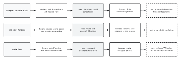
Holographic renormalization fixes divergences but leaves declared finite schemes, boundary conditions, and contact terms in the physical answer. Each row pairs a diagnostic with the strongest supported conclusion and an explicitly unsupported promotion. The diagram is an original schematic and is not to scale.

Accessible figure data (JSON)

Claim-domain comparison

The table below gives a screen-reader-friendly comparison of three representative claims. It keeps the required declaration, approximation status, evidence timing, counterevidence, falsifier, failure condition, and licensed conclusion in one reading order.

Representative claim domains and validity boundaries for Holographic Renormalization and Radial Dynamics

Claim object	State, ensemble, and conventions	Approximation, status, and evidence timing	Uncertainty and counterevidence	Falsifier	Failure condition	Licensed conclusion
divergent on-shell action	Declare radial coordinate and induced fields; use the volume conventions unless the page states a local replacement.	Model-specific calculation or conditional result. Control chain: Fefferman-Graham cutoff data → radial Hamilton-Jacobi recursion → local and finite counterterms → one-point functions and Ward identities → renormalized observable. Sources are cited on the destination page; literature checked through 10 August 2026.	Track omitted corrections, alternate branches, and competing definitions. A failed “Hamilton-Jacobi cancellation” check is counterevidence to the promoted claim.	Hamilton-Jacobi cancellation	scheme-independent finite contact terms	finite variational problem
one-point function	Declare source normalization and counterterm action; use the volume conventions unless the page states a local replacement.	Model-specific calculation or conditional result. Control chain: Fefferman-Graham cutoff data → radial Hamilton-Jacobi recursion → local and finite counterterms → one-point functions and Ward identities → renormalized observable. Sources are cited on the destination page; literature checked through 10 August 2026.	Track omitted corrections, alternate branches, and competing definitions. A failed “Ward and anomaly identities” check is counterevidence to the promoted claim.	Ward and anomaly identities	a bare bulk coefficient	renormalized response in one scheme
radial flow	Declare cutoff surface and boundary conditions; use the volume conventions unless the page states a local replacement.	Model-specific calculation or conditional result. Control chain: Fefferman-Graham cutoff data → radial Hamilton-Jacobi recursion → local and finite counterterms → one-point functions and Ward identities → renormalized observable. Sources are cited on the destination page; literature checked through 10 August 2026.	Track omitted corrections, alternate branches, and competing definitions. A failed “canonical transformation check” check is counterevidence to the promoted claim.	canonical transformation check	ordinary Wilsonian RG without qualifications	radial evolution of data

Download the structured table data (JSON).

References

• de Haro, Sebastian, Sergey N. Solodukhin, and Kostas Skenderis. “Holographic Reconstruction of Spacetime and Renormalization in the AdS/CFT Correspondence.” Communications in Mathematical Physics 217, 595–622 (2001). DOI; arXiv:hep-th/0002230.
• Papadimitriou, Ioannis. “Holographic Renormalization as a Canonical Transformation.” Journal of High Energy Physics 2010, 014 (2010). DOI; arXiv:1007.4592.
• Skenderis, Kostas. “Lecture Notes on Holographic Renormalization.” Classical and Quantum Gravity 19, 5849–5876 (2002). DOI; arXiv:hep-th/0209067.