Higher-Derivative and Quantum Entropy Corrections

Subleading black-hole entropy is a sharper microscopic test than the area law. Fix a protected microscopic quantity, a fixed-charge single-center horizon sector, and an integral large-charge family. The charge map, chamber, and ensemble must agree before local higher-derivative saddle corrections, nonzero-mode determinants, zero-mode measures, and inverse-transform Jacobians can be compared order by order. This page carries out one such logarithmic match for four-dimensional quarter-BPS dyons and then deliberately omits the zero-mode measure: the leading entropy survives, but logarithmic precision fails.

Required background. Noether-Charge Entropy and Higher-Curvature Terms supplies the macroscopic entropy functional; Attractor Mechanism and Charge-Only Entropy supplies the regular charge-fixed saddle.

Helpful background. One-Loop Graviton EFT supplies determinant and renormalization power counting; Marginal Stability, Chambers, and Wall Crossing supplies chamber control.

The detailed Noether-charge derivation remains on the first prerequisite. Here the local analysis is restricted to a regular extremal near-horizon saddle for which the entropy-function construction applies. The quantum calculation is restricted further to a protected four-dimensional $\mathcal N=4$ sector; it is not a claim about generic non-BPS black holes.

A lattice-compatible large-charge comparison

Let $\Gamma(n)$ be a family of allowed lattice charges with $n\to\infty$, while the compactification, Newton constant, specified arithmetic orbit data, chamber, and boundary conditions remain fixed. For a signed protected quantity $\mathcal I(\Gamma)$, define

$$S_{\rm micro}(n)=\log\left\lvert\mathcal I(\Gamma(n))\right\rvert.$$

Only after choosing the family is it meaningful to speak about the coefficient of $\log n$. A useful schematic expansion is

$$S(n) =S_0\bigl(\Gamma(n)\bigr) +\sum_r S_{{\rm local},r}\bigl(\Gamma(n)\bigr) +a\log n+b+\cdots .$$

The powers hidden in the local terms and in the remainder are theory- and trajectory-dependent. In a four-dimensional large black hole, for example, a four-derivative term is often $O(n^0)$ and a six-derivative term $O(n^{-2})$, but this is not a universal theorem. Alternate saddles can instead be exponentially suppressed. Keeping $S_0$ as the exact function of $\Gamma(n)$ prevents a subleading term generated merely by the chosen lattice family from being misidentified as a quantum correction.

The comparison must specify the following data before any coefficients are equated:

• the protected trace or degeneracy, including its sign convention;
• the integer microscopic charges and the corresponding asymptotic or near-horizon charges;
• the single-center branch, contour, chamber, and treatment of exterior degrees of freedom;
• the fixed-charge, mixed, or potential ensemble and every transformed variable;
• the effective action, renormalization scale, massless spectrum, ghosts, boundary conditions, and regulator;
• the order retained and the first unresolved remainder.

The microscopic entropy comparison contract develops this bookkeeping in general. The purpose here is to show how it controls an actual subleading calculation.

Local terms, determinants, and collective coordinates

Different contributions can have the same asymptotic size even though they arise from different calculations. A consistent split is therefore made at a declared Wilsonian scale and recombined before a physical coefficient is reported.

Contribution	Possible asymptotic signature	Data needed for a reproducible result
Local higher-derivative action	powers, constants, and sometimes running logarithms	renormalized couplings, field basis, corrected saddle, and charge convention
Nonzero massless modes	one-loop logarithms and constants	complete massless spectrum, gauge fixing, ghosts, boundary conditions, and regulator
Zero modes	collective-coordinate logarithms	zero-mode norms, symmetry parameters, integration ranges, and Jacobians
Ensemble transform	Hessian and measure logarithms	polarization, contour, periodicities, normalized measure, and determinant with zero directions removed
Charge and sector map	can shift an earlier asymptotic order	quantized, Page, Maxwell, or flux charges; exterior modes; chamber; and center decomposition

Massive fields can renormalize local Wilsonian operators. They do not generally determine the infrared logarithm in the simultaneous large-charge limit, but they can affect the $O(1)$ term. Counting a loop once through a running local coupling and again through the determinant that generated it would double-count the same physics.

Local corrections at an extremal saddle

For an $AdS_2\times S^2$ near-horizon ansatz, let $x^A$ collect the constant scalars, radii, and electric fields $e^I$, while the magnetic fluxes $p^I$ are fixed. For a local covariant Lagrangian scalar $\mathcal L$, define

$$f(x,p)=\int_{S^2}d\theta\,d\varphi\,\sqrt{-g}\,\mathcal L, \qquad q_I=\frac{\partial f}{\partial e^I},$$

and the entropy function

$$\mathcal E(q,p;x)=2\pi\bigl(q_Ie^I-f(x,p)\bigr).$$

Its stationary equations $\partial_A\mathcal E=0$ determine the near-horizon data, and its stationary value is the local Wald entropy. This is the extremal algebraic form of the Noether-charge result Sen 2005, §§ 2–3, especially eqs. (2.14), (2.17)–(2.18), and (3.1)–(3.5), Open PDF.

The first-order correction has a useful simplification. Write

$$\mathcal E=\mathcal E_0+\varepsilon\mathcal E_1, \qquad x_*^A=x_0^A+\varepsilon x_1^A+O(\varepsilon^2),$$

where $\partial_A\mathcal E_0(x_0)=0$. Then

$$S_{\rm local} =\mathcal E(x_*) =\mathcal E_0(x_0) +\varepsilon\mathcal E_1(x_0) +O(\varepsilon^2).$$

The correction to the fields is necessary to construct the corrected solution, but it drops out of the entropy at first order because the unperturbed saddle is stationary. This does not license use of an incomplete action: all operators contributing at the requested order must still be included.

The inherited Noether-charge convention matters. For a stationary bifurcate Killing horizon and a Lagrangian containing derivatives of curvature, the entropy uses the Euler derivative $E_R^{\mu\nu\rho\sigma}$ rather than only $\partial\mathcal L/\partial R_{\mu\nu\rho\sigma}$; Iyer and Wald 1994, eq. (31), p. 7; eq. (53), p. 10; and Theorem 6.1 with eq. (93), pp. 16–17, Open PDF gives the covariant construction. A strictly extremal horizon has no bifurcation surface. Here its entropy is defined by the smooth nonextremal limit described in Sen 2005, § 1, p. 2, Open PDF and evaluated on the regular $AdS_2\times S^2$ saddle with the entropy function. Noncovariant gravitational Chern–Simons terms require a modified treatment Tachikawa 2007, §§ 2–3, Open PDF.

The fixed-charge quantum entropy function

The quantum entropy function promotes the extremal saddle to a path integral. With fixed electric charges $q_I$ and magnetic fluxes $p^I$,

$$d_{\rm hor}(q,p) =\left\langle \exp\!\left[-iq_I\oint_{\partial AdS_2}A^I\right] \right\rangle_{AdS_2}^{\rm finite}.$$

The superscript “finite” means that the boundary-length divergence of regulated Euclidean $AdS_2$ has been removed. The dominant electric-field mode is held fixed, so this object is already in a fixed-charge sector; the constant boundary-potential mode fluctuates. An additional ensemble Hessian must not be appended unless one separately starts from a potential-space generating function and transforms it. These boundary conditions and the Wilson-line insertion are derived in Sen 2009, eq. (1.3), §§ 3–4, Open PDF.

Schematically,

$$\log\left\lvert d_{\rm hor}\right\rvert =S_{\rm local} +\log Z_{\rm nonzero} +\log Z_{\rm zero} +\cdots .$$

The prime on a nonzero-mode determinant is not decorative: every zero eigenfunction must be removed. A true zero mode has no Gaussian restoring force. One changes variables from its normalized field coefficient to a collective coordinate—such as a gauge, diffeomorphism, or supersymmetry parameter—and includes the resulting scale-dependent Jacobian. Sen 2012, §§ 2.2–2.5, especially eq. (2.22), Open PDF shows explicitly how subtracting a zero mode from the determinant and then integrating it as a collective coordinate give different terms.

An inverse transform at logarithmic order

Suppose instead that a microscopic or thermodynamic quantity is first known in potential space and that a fixed-charge coefficient is obtained from

$$\mathcal I(\Gamma) =\int_{\mathcal C}d^m\phi\, \mu(\phi;n)\, \exp\!\bigl[\Phi(\phi;\Gamma)\bigr].$$

Choose a steepest-descent contour $\mathcal C$ through a nondegenerate saddle $\phi_*$. Let $H_\perp$ be the quadratic form restricted to the nonzero steepest-descent directions. Then

$$\left\lvert\mathcal I(\Gamma)\right\rvert \simeq \left\lvert\mu(\phi_*;n)e^{\Phi(\phi_*;\Gamma)}\right\rvert \frac{(2\pi)^{m_\perp/2}} {\sqrt{\left\lvert\det{}'H_\perp\right\rvert}}.$$

If

$$\mu(\phi_*;n)\sim n^\beta, \qquad \left\lvert h_i(H_\perp)\right\rvert\sim n^{\kappa_i},$$

then the transform changes the logarithmic coefficient by

$$\Delta a_{\rm transform} =\beta-\frac12\sum_i\kappa_i.$$

The often quoted $-m\kappa/2$ follows only when every eigenvalue has the same scaling and the measure has no power of $n$. A complex or thermodynamically unstable saddle requires contour rotation, not an absolute-value Gaussian on the original real contour. A zero eigenvalue is excluded from $\det{}'H_\perp$ and treated by a collective coordinate or by higher-order saddle analysis. The normalized contour, measure, pole residues, and Jacobians are part of the answer; a bare Hessian determinant is coordinate-dependent. Sen 2013, § 3.1, eqs. (3.5)–(3.12) and footnote 10, Open PDF gives an explicit black-hole ensemble transform.

A protected quarter-BPS N=4 match

Consider type II string theory on $K3\times T^2$, equivalently heterotic string theory on $T^6$, at a generic Abelian point. Its four-dimensional $\mathcal N=4$ supergravity contains $m=22$ matter multiplets in addition to the gravity multiplet.

The protected object and its horizon sector

A quarter-BPS state preserves four of the sixteen supercharges and breaks twelve. Its protected sixth helicity trace is

$$B_6(Q,P) =\frac1{6!}\operatorname{Tr}_{Q,P} \!\left[(-1)^{2J_3}(2J_3)^6\right].$$

The six powers of $2J_3$ saturate the six pairs of Goldstino zero modes generated by the broken supersymmetries. Define $\mathcal I_6=-B_6$ in the single-center convention and compare $\log\lvert\mathcal I_6\rvert$ with the fixed-charge horizon result.

Two kinds of zero mode must not be conflated. Gauge, diffeomorphism, and gravitino zero modes inside the $AdS_2$ path integral alter its logarithm through collective-coordinate Jacobians. For the exterior sector, use the same normalized trace,

$$B_{6,{\rm hair}}(\Gamma) \equiv \frac1{6!}\operatorname{Tr}_{{\rm hair},\Gamma} \!\left[(-1)^{2J_3}(2J_3)^6\right].$$

Exterior Goldstino hair then relates the horizon degeneracy to the asymptotic helicity trace:

$$B_6(Q,P) =\sum_{\Gamma_{\rm hor}+\Gamma_{\rm hair}=(Q,P)} d_{\rm hor}(\Gamma_{\rm hor}) B_{6,{\rm hair}}(\Gamma_{\rm hair}).$$

When the only exterior modes in the single-center sector are the neutral universal Goldstinos, $B_{6,{\rm hair}}=(-1)^3=-1$ and $\mathcal I_6^{\rm single}=d_{\rm hor}$. Additional hair must be deconvolved before comparison. This index–horizon factorization is derived in Dabholkar et al. 2011, § 2, especially eqs. (2.1), (2.4)–(2.6), (2.8)–(2.9), and the paragraph following eq. (2.9), Open PDF.

An exact torsion-one charge family

Let $Q,P\in\Gamma^{6,22}$ and define

$$\Delta=Q^2P^2-(Q\mathbin{\cdot}P)^2.$$

A regular large single-center branch requires $Q^2>0$, $P^2>0$, and $\Delta>0$. Literal multiplication of both lattice vectors by the same integer changes the discrete dyon torsion

$$r(Q,P)=\gcd_{i,j}\bigl(Q_iP_j-Q_jP_i\bigr).$$

This arithmetic invariant labels distinct dyon sectors: the torsion-one coefficient uses the basic $1/\Phi_{10}$ partition function, whereas higher-torsion sectors require additional divisor data Banerjee, Sen, and Srivastava 2008, introduction, pp. 1–2, and eqs. (1)–(4), Open PDF.

To keep the dyon torsion fixed at $r=1$, choose a $U\oplus U$ sublattice with null basis vectors satisfying $e_i\mathbin{\cdot}f_j=\delta_{ij}$ and define, for positive integer $n$,

$$\begin{aligned} Q_n&=n e_1+(n+1)f_1+n e_2+(n-1)f_2,\\ P_n&=(1-n)e_1-nf_1+n e_2+(2n+1)f_2. \end{aligned}$$

The $(e_1,f_1)$ wedge minor is

$$n(-n)-(n+1)(1-n)=-1,$$

so $r(Q_n,P_n)=1$ for every $n$. Direct contraction gives

$$Q_n^2=4n^2, \qquad P_n^2=6n^2, \qquad Q_n\mathbin{\cdot}P_n=n^2+1,$$

and therefore

$$\Delta_n=23n^4-2n^2-1, \qquad \log\Delta_n=4\log n+\log 23+O(n^{-2}).$$

The leading axion–dilaton saddle remains in the interior,

$$\tau_*(n) =\frac{Q_n\mathbin{\cdot}P_n+i\sqrt{\Delta_n}}{P_n^2} \longrightarrow \frac{1+i\sqrt{23}}6.$$

This family supplies the promised control parameter without changing the dyon torsion.

The microscopic logarithm

In the attractor chamber, the torsion-one single-center contribution is extracted from the exact Siegel-modular inverse transform

$$\mathcal I_6(Q,P) =(-1)^{Q\cdot P+1} \int_{\mathcal C_{\rm attr}} d\rho\,d\sigma\,dv\, \frac{ \exp\!\left[-\pi i\left(\rho P^2+\sigma Q^2+2vQ\mathbin{\cdot}P\right)\right] }{\Phi_{10}(\rho,\sigma,v)}.$$

This sign-adjusted fixed-charge coefficient and its $\Phi_{10}$ inverse transform are written explicitly in Dabholkar et al. 2011, eq. (5.28), p. 42, Open PDF. The displayed $\rho P^2+\sigma Q^2$ assignment, periods, and attractor contour follow Banerjee, Jatkar, and Sen 2009, eqs. (2.1)–(2.6), pp. 3–4, and eq. (2.9), p. 5, Open PDF. The torsion-one condition is what permits the bare $1/\Phi_{10}$ integrand rather than a higher-torsion divisor sum. The contour is part of the observable: it selects the attractor chamber and separates the single-center saddle from wall-dependent multicenter residues. The dominant quadratic divisor reduces this integral to a two-variable saddle. For $K3\times T^2$, use the standard $4\pi K_0=1$ normalization; changing $K_0$ shifts only the charge-independent constant omitted here. The first correction is then

$$\begin{aligned} \log\left\lvert\mathcal I_6(Q,P)\right\rvert &=\pi\sqrt\Delta+S^{(1)}(\tau_*)+O(\Delta^{-1/2}),\\ S^{(1)}(\tau) &=-24\log\left\lvert\eta(\tau)\right\rvert^2 -12\log\bigl(2\operatorname{Im}\tau\bigr). \end{aligned}$$

This explicitly real form follows from $\eta(-\bar\tau)=\overline{\eta(\tau)}$ and Banerjee, Jatkar, and Sen 2009, eqs. (3.13)–(3.14), Open PDF.

Along the explicit family, $\tau_*(n)$ approaches a finite interior point, so $S^{(1)}(\tau_*)=O(1)$. Consequently,

$$S_{\rm micro}(n) =\pi\sqrt{\Delta_n} +0\cdot\log n +O(1).$$

At the residue-reduced saddle, the charge-dependent double-pole prefactor scales as $n^2$, while the two-dimensional Gaussian has $\det H\sim n^4$ and contributes $n^{-2}$. Their logarithms cancel. This is a concrete microscopic example of why the full measure, not the Hessian alone, defines an ensemble correction. The contour, saddle, measure, and expansion are given in Banerjee, Jatkar, and Sen 2009, §§ 2.1–2.2 and § 3, Open PDF.

The macroscopic logarithm

The regular near-horizon geometry is $AdS_2\times S^2$ with common scale $a$ satisfying

$$\frac{a^2}{G_4}=\sqrt{\Delta_n}, \qquad S_{\rm BH}^{(0)}=\pi\sqrt{\Delta_n}.$$

The fixed-charge quantum entropy function includes the determinants of all massless fields and their ghosts, with zero modes removed and integrated separately. For four-dimensional $\mathcal N=4$ supergravity with $m$ matter multiplets, the published one-loop result is

$$\Delta S_{\rm nonzero} =\frac{6+m}{4}\log\Delta, \qquad \Delta S_{\rm zero} =-\frac{6+m}{4}\log\Delta.$$

For $K3\times T^2$, $m=22$, so the comparison is

Contribution	Coefficient of $\log\Delta_n$	Coefficient of $\log n$	Meaning
Nonzero massless modes	$+7$	$+28$	determinant with zero eigenfunctions removed
Zero modes	$-7$	$-28$	collective-coordinate Jacobians
Macroscopic total	$0$	$0$	fixed-charge horizon result
Microscopic $\log\lvert\mathcal I_6\rvert$	$0$	$0$	same charge family and single-center chamber

The vanishing total is therefore not an absence of quantum fluctuations. There are $6+22=28$ gauge fields. For each gauge field, the regularized collective-coordinate integral over its $AdS_2$ zero-mode tower contributes $-\log a=-\tfrac14\log\Delta+O(1)$; the net graviton and gravitino zero-mode terms cancel, giving $-7\log\Delta$ in total. The nonzero modes give the opposite $+7\log\Delta$. These coefficients and the microscopic asymptotic are reported in Banerjee et al. 2011, eq. (1.1), Table 1, §§ 3 and 7, Open PDF.

The figure makes the cancellation and its failure control visible. Inspect the signed coefficients rather than only the zero at the end.

On a narrow screen, swipe or use the Left and Right arrow keys to pan across the figure. Home and End move to its edges. A full-size link is also available.

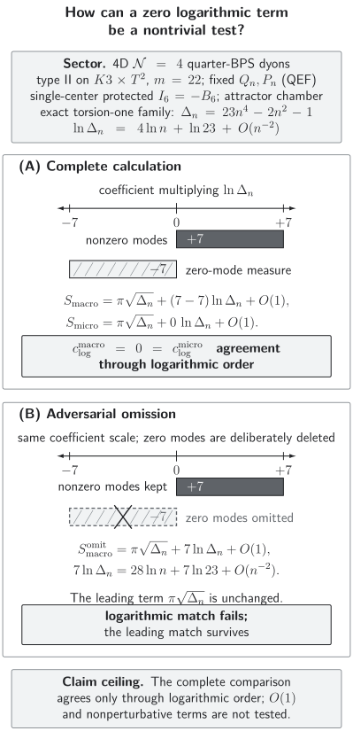
For the torsion-one quarter-BPS $K3\times T^2$ family, nonzero massless modes contribute $+7\log\Delta_n$ and the zero-mode collective-coordinate measure contributes $-7\log\Delta_n$. Their exact cancellation matches the protected fixed-charge microscopic asymptotic, which has no logarithmic term. The failure control omits zero modes and leaves a false $+7\log\Delta_n=28\log n+O(1)$ while preserving the leading $\pi\sqrt{\Delta_n}$. Coefficient lengths are quantitative; the comparison establishes agreement only through logarithmic order.

Combining both sides,

$$S_{\rm macro}(n) =\pi\sqrt{\Delta_n} +\bigl(7-7\bigr)\log\Delta_n +O(1) =S_{\rm micro}(n)+O(1).$$

The equality displayed here means equality of the leading and logarithmic coefficients. It does not assert equality of the unresolved constants.

The zero-mode omission falsifies logarithmic precision

Now perform the manifestly wrong calculation: keep every nonzero eigenvalue but discard the collective-coordinate integral. The result becomes

$$S_{\rm macro}^{\rm wrong}(n) =\pi\sqrt{\Delta_n} +7\log\Delta_n +O(1) =\pi\sqrt{\Delta_n} +28\log n +O(1).$$

The leading area term still agrees with the microscopic saddle, but the coefficient of $\log n$ differs by $28$. The strongest surviving statement is therefore a leading-order entropy match; agreement through logarithmic order has been falsified.

There is a parallel microscopic failure. Keeping the two-dimensional Gaussian, whose determinant contributes $-2\log n$, while dropping the charge-dependent double-pole residue that contributes $+2\log n$ creates a spurious microscopic logarithm. Both failures have the same lesson: a determinant is not a complete measure.

Changing the scaling limit also changes the question. The result above uses simultaneous large-charge scaling. In the Cardy limit, where one charge grows while the others remain fixed, the same $K3\times T^2$ theory has a microscopic coefficient $-6\log\Delta$, not zero Banerjee et al. 2011, § 1 after eq. (1.3), Open PDF. The two answers concern different asymptotic regimes and do not contradict one another.

Charge shifts can enter before the logarithm

Microscopic integer charges, asymptotic conserved charges, near-horizon fluxes, and Page or Maxwell charges need not coincide in theories with Chern–Simons couplings or induced lower-dimensional charges. Their properties differ, so the charge map must be fixed before expanding Marolf 2001, §§ 2–4, pp. 3–9, Open PDF.

A one-variable model shows why an apparently harmless constant shift can matter. Suppose

$$q_{\rm micro}=q_{\rm macro}+c, \qquad S_0=Aq_{\rm macro}^2, \qquad q_{\rm micro}=n\widehat q.$$

Then

$$S_0 =A(n\widehat q-c)^2 =An^2\widehat q^{\,2} -2Acn\widehat q +Ac^2.$$

An $O(1)$ charge shift has generated an $O(n)$ entropy term, parametrically earlier than $\log n$. Calling it a small finite-charge ambiguity would corrupt every later comparison.

The safe order of operations is:

1. identify the same quantized charge, protected trace, center decomposition, chamber, and ensemble on both sides;
2. evaluate all local terms at the appropriate corrected saddle and in one renormalization scheme;
3. compute the nonzero-mode determinant with complete gauge fixing and ghosts;
4. integrate zero modes with normalized collective coordinates;
5. perform any required ensemble transform with its contour, residues, and measure; and
6. expand both answers along the same integral charge family and state the unresolved remainder.

What the logarithmic match establishes

The controlled result is conditional and specific: for the stated torsion-one sequence, the attractor-contour single-center helicity trace and the fixed-charge quantum entropy function agree in their leading and logarithmic coefficients after all exterior hair is deconvolved. The direct identification $\mathcal I_6^{\rm single}=d_{\rm hor}$ uses the universal-Goldstino-only hypothesis stated above. The macroscopic zero is a nontrivial cancellation between a $+28\log n$ nonzero-mode contribution and a $-28\log n$ zero-mode measure. The result is analytic, so there is no numerical fitting uncertainty in these coefficients.

The comparison does not determine the full $O(1)$ constant, exponentially suppressed saddles, an exact finite-charge value, an absolute unprotected degeneracy, a different chamber including multicenter states, the Cardy limit, or a generic non-BPS entropy. Those require additional data rather than a stronger interpretation of the calculation already performed.

Common pitfalls

Calling an index a degeneracy. $B_6$ is a signed helicity trace. The horizon degeneracy can be related to it only after the Goldstino and any additional exterior modes have been accounted for.

Reading zero as “nothing happened.” The $\mathcal N=4$ logarithm vanishes because two nonzero contributions cancel. Deleting either one changes the precision result.

Putting zero modes back into the determinant. A zero eigenvalue invalidates the Gaussian approximation. Remove it from $\det{}'$ and derive the collective-coordinate measure separately.

Adding a Hessian to an already fixed-charge path integral. The quantum entropy function already fixes the charges through its $AdS_2$ boundary condition. A Hessian appears only when a separately defined potential-space object is transformed.

Using only the Hessian of an inverse transform. Pole residues and charge-dependent measures can cancel its logarithm, as they do in the microscopic dyon integral. The contour and full measure are part of the observable.

Scaling lattice vectors without checking discrete invariants. Literal multiplication can change the dyon torsion. Use a valid integral family and hold the specified arithmetic invariants fixed; the sequence above keeps $r(Q_n,P_n)=1$.

Mixing simultaneous scaling with a Cardy limit. Their logarithmic coefficients need not agree because different charge ratios and saddle regions are being probed.

Claiming finite-charge precision from a logarithmic match. Agreement through $\log n$ leaves the constant and smaller terms unresolved. State that ceiling explicitly.

Exercises

1. Verify the integral charge family

Using $e_i^2=f_i^2=0$ and $e_i\mathbin{\cdot}f_j=\delta_{ij}$, verify $Q_n^2$, $P_n^2$, $Q_n\mathbin{\cdot}P_n$, $\Delta_n$, and the torsion-one minor. Then derive the first two terms of $\log\Delta_n$.

Solution

For a vector $x=a_1e_1+b_1f_1+a_2e_2+b_2f_2$, $x^2=2(a_1b_1+a_2b_2)$. Hence

$$Q_n^2=2\bigl[n(n+1)+n(n-1)\bigr]=4n^2,$$

and

$$P_n^2=2\bigl[(1-n)(-n)+n(2n+1)\bigr]=6n^2.$$

The mixed contraction is

$$Q_n\mathbin{\cdot}P_n =n(-n)+(n+1)(1-n)+n(2n+1)+(n-1)n =n^2+1.$$

Therefore $\Delta_n=24n^4-(n^2+1)^2=23n^4-2n^2-1$. The $(e_1,f_1)$ wedge minor equals $-1$, so the gcd of all minors is one. Finally,

$$\log\Delta_n =4\log n+\log 23 +\log\!\left(1-\frac{2}{23n^2}-\frac{1}{23n^4}\right) =4\log n+\log23+O(n^{-2}).$$

2. Evaluate a first-order local entropy correction

Let $\mathcal E(x;\varepsilon)=\mathcal E_0(x)+\varepsilon\mathcal E_1(x)$ and $x_*=x_0+\varepsilon x_1+O(\varepsilon^2)$, with $\partial_A\mathcal E_0(x_0)=0$. Show that $x_1$ does not enter the entropy at first order.

Solution

Taylor expansion gives

$$\mathcal E(x_*;\varepsilon) =\mathcal E_0(x_0) +\varepsilon x_1^A\partial_A\mathcal E_0(x_0) +\varepsilon\mathcal E_1(x_0) +O(\varepsilon^2).$$

The middle term vanishes by stationarity, leaving $\mathcal E_0(x_0)+\varepsilon\mathcal E_1(x_0)+O(\varepsilon^2)$.

3. Expose the zero-mode failure

Insert $m=22$ into the general $\mathcal N=4$ coefficients. Convert the result from $\log\Delta_n$ to $\log n$, and repeat the calculation after omitting zero modes.

Solution

Since $(6+m)/4=28/4=7$,

$$\Delta S_{\rm nonzero}=+7\log\Delta_n, \qquad \Delta S_{\rm zero}=-7\log\Delta_n.$$

Their sum is zero. Because $\log\Delta_n=4\log n+O(1)$, the separate coefficients are $+28$ and $-28$ in the $\log n$ convention. Omitting zero modes leaves the false term $+28\log n+O(1)$, so only the leading area match survives.

4. Include the full Gaussian measure

Suppose $\mu(\phi_*;n)\sim n^\beta$ and the nonzero Hessian eigenvalues scale as $\lvert h_i\rvert\sim n^{\kappa_i}$. Derive the transform contribution to the logarithmic coefficient. Evaluate it for $\beta=1$ and $\kappa=(2,1,1)$.

Solution

The measure supplies $\beta\log n$, while the Gaussian denominator supplies $-\tfrac12\sum_i\kappa_i\log n$. Thus

$$\Delta a_{\rm transform} =\beta-\frac12\sum_i\kappa_i.$$

For the stated values, $\Delta a=1-\tfrac12(2+1+1)=-1$.

5. Diagnose a flat Gaussian direction

One Hessian eigenvalue vanishes. Why is $\det H=0$ not an infinite entropy correction, and what replaces the Gaussian integral in that direction?

Solution

The quadratic approximation contains no restoring term along that direction, so the Gaussian formula is inapplicable rather than divergent physics. Remove the direction from $\det{}'H$. If it is an exact zero direction—whether symmetry-generated or a genuine modulus—replace the Gaussian by the correctly normalized group or moduli integral, including its range and Jacobian. If only the quadratic term vanishes, retain the first nonzero higher-order term and redo the saddle approximation.

6. Track a constant charge shift

Let $q_{\rm micro}=q_{\rm macro}+c$ and $S_0=Aq_{\rm macro}^2$. If $q_{\rm micro}=n\widehat q$, determine the orders generated by $c$ and explain why the charge map precedes the logarithmic comparison.

Solution

Substitution gives

$$S_0=A(n\widehat q-c)^2 =An^2\widehat q^{\,2}-2Acn\widehat q+Ac^2.$$

The constant charge shift produces an $O(n)$ term and an $O(1)$ term. The $O(n)$ term occurs parametrically before the logarithm, while the $O(1)$ term occurs after it; the earlier mismatch alone is enough to make a logarithmic comparison uninterpretable until the charge map is fixed.

Continue to Supersymmetric Localization and Quantum Entropy-Function Tests for the conditional reduction of the fixed-charge $AdS_2$ path integral to a finite-dimensional integral, including its contour and measure.

The chapter overview contains the structure diagram and validity and failure diagram. They are embedded there once so that their shared chapter-level context is not repeated on every article.

For the chapter-wide comparison of assumptions, counterevidence, falsifiers, and claim ceilings, see the claim-domain table.

References

• Banerjee, Nabamita, Dileep P. Jatkar, and Ashoke Sen. “Asymptotic Expansion of the $\mathcal N=4$ Dyon Degeneracy.” Journal of High Energy Physics 05 (2009): 121. DOI. Open PDF.
• Banerjee, Shamik, Ashoke Sen, and Yogesh K. Srivastava. “Partition Functions of Torsion $>1$ Dyons in Heterotic String Theory on $T^6$.” Journal of High Energy Physics 05 (2008): 098. DOI. Open PDF.
• Banerjee, Shamik, Rajesh Kumar Gupta, Ipsita Mandal, and Ashoke Sen. “Logarithmic Corrections to $\mathcal N=4$ and $\mathcal N=8$ Black Hole Entropy: A One Loop Test of Quantum Gravity.” Journal of High Energy Physics 11 (2011): 143. DOI. Open PDF.
• Dabholkar, Atish, João Gomes, Sameer Murthy, and Ashoke Sen. “Supersymmetric Index from Black Hole Entropy.” Journal of High Energy Physics 04 (2011): 034. DOI. Open PDF.
• Iyer, Vivek, and Robert M. Wald. “Some Properties of Noether Charge and a Proposal for Dynamical Black Hole Entropy.” Physical Review D 50 (1994): 846–864. DOI. Open PDF.
• Marolf, Donald. “Chern–Simons Terms and the Three Notions of Charge.” In Quantization, Gauge Theory, and Strings: Proceedings of the International Conference Dedicated to the Memory of Efim Fradkin, edited by A. Semikhatov, M. Vasiliev, and V. Zaikin, 312–320. Moscow: Scientific World, 2001. Open PDF.
• Sen, Ashoke. “Black Hole Entropy Function and the Attractor Mechanism in Higher Derivative Gravity.” Journal of High Energy Physics 09 (2005): 038. DOI. Open PDF.
• Sen, Ashoke. “Quantum Entropy Function from $AdS_2/CFT_1$ Correspondence.” International Journal of Modern Physics A 24 (2009): 4225–4244. DOI. Open PDF.
• Sen, Ashoke. “Logarithmic Corrections to Rotating Extremal Black Hole Entropy in Four and Five Dimensions.” General Relativity and Gravitation 44 (2012): 1947–1991. DOI. Open PDF.
• Sen, Ashoke. “Logarithmic Corrections to Schwarzschild and Other Non-Extremal Black Hole Entropy in Different Dimensions.” Journal of High Energy Physics 04 (2013): 156. DOI. Open PDF.
• Tachikawa, Yuji. “Black Hole Entropy in the Presence of Chern–Simons Terms.” Classical and Quantum Gravity 24 (2007): 737–744. DOI. Open PDF.