Exchange Witten Diagrams and Conformal Blocks

A tree-level scalar exchange Witten diagram is generally not one conformal block. In one Euclidean $12\to34$ channel, the full AdS integral solves an inhomogeneous Casimir equation: the exchanged field supplies one single-trace family, while the collapsed Green-function source supplies two scalar double-trace towers, one from each external pair. A geodesic Witten object isolates the single conformal family; the ordinary exchange diagram does not.

In the semiclassical large-$N$ organization, “single trace” corresponds to a one-particle bulk sector and “double trace” to a two-particle sector; these names need not be literal trace counts at finite $N$.

This page works in Euclidean AdS$_{d+1}$ with radius $L$, separated boundary insertions, standard quantization, scalar external and exchanged fields, nonderivative cubic vertices, and a fixed tree-level bulk action. Alternate quantization, derivative vertices, internal spin, Lorentzian orderings, and loops require additional data.

Required background. AdS propagators supplies the normalized kernels and Green equation. Blocks and Casimir equations supplies the boundary Casimir and the physical-versus-shadow boundary condition.

Helpful background. Conformal OPE data supplies the spectral interpretation. D’Hoker and Freedman’s teaching treatment gives a broader route from normalized AdS fields to boundary correlators D’Hoker and Freedman 2004, §§ 6.2–6.3 and 7.5–7.12, pp. 52–55 and 68–78.

The scalar exchange kernel

Let $x_i$ be four boundary points, and write $K_i(X)=K_{\Delta_i}(X;x_i)$ for the normalized bulk-to-boundary kernel. A scalar $\chi$ of dimension $\Delta_\chi$ has

$$C_\chi:=m_\chi^2L^2=\Delta_\chi(\Delta_\chi-d), \qquad (-\Box_X+m_\chi^2)G_\chi(X,Y)=\delta_g(X,Y),$$

where $\delta_g(X,Y)=\delta^{d+1}(X-Y)/\sqrt{g(X)}$. The standard-quantized Euclidean Green function is symmetric, regular away from coincidence, and normalizable at the boundary. For cubic interactions $g_{12\chi}\phi_1\phi_2\chi$ and $g_{34\chi}\phi_3\phi_4\chi$, define $\lambda=g_{12\chi}g_{34\chi}$ and

$$\begin{aligned} \mathcal E_s(x_i)={}&\lambda \int_{\mathrm{AdS}}d\mu_X\int_{\mathrm{AdS}}d\mu_Y\, K_1(X)K_2(X)G_\chi(X,Y)K_3(Y)K_4(Y),\\ d\mu_X:={}&d^{d+1}X\sqrt{g(X)}. \end{aligned}$$

This is a position-dependent contribution to the connected four-point function, not yet a function only of cross-ratios. With $\Delta_{ij}=\Delta_i-\Delta_j$, separate the external covariance as

$$\begin{aligned} \mathcal E_s(x_i)&=\mathcal P_{\Delta_i}(x_i)\,\mathcal W_s(u,v),\\ \mathcal P_{\Delta_i}(x_i)&= \frac{1}{(x_{12}^2)^{(\Delta_1+\Delta_2)/2}(x_{34}^2)^{(\Delta_3+\Delta_4)/2}} \left(\frac{x_{24}^2}{x_{14}^2}\right)^{\Delta_{12}/2} \left(\frac{x_{14}^2}{x_{13}^2}\right)^{\Delta_{34}/2},\\ u&=\frac{x_{12}^2x_{34}^2}{x_{13}^2x_{24}^2}, \qquad v=\frac{x_{14}^2x_{23}^2}{x_{13}^2x_{24}^2}. \end{aligned}$$

Liu gives the normalized double integral and its OPE pole families in Liu 1999, § 2, eqs. (2.2)–(2.5) and (2.16), pp. 7–10. Normalizations must not be mixed across sources: some authors absorb constants into $K$, $G_\chi$, or the cubic couplings.

Throughout, $\mathcal B_{\Delta,\ell}(x_i)=\mathcal P_{\Delta_i}(x_i)g_{\Delta,\ell}(u,v)$ denotes the physical block contribution with its external prefactor, while $g_{\Delta,\ell}$ is the reduced block.

The Casimir turns exchange into a contact source

Set $F_{12}(X)=K_1(X)K_2(X)$ and $F_{34}(Y)=K_3(Y)K_4(Y)$. In the site’s Casimir-sign convention,

$$\mathcal C_{12}F_{12}(X)=L^2\Box_XF_{12}(X), \qquad \mathcal C_{12}=\frac12(J_1+J_2)_{AB}(J_1+J_2)^{AB}.$$

Here $J$ denotes the site’s Hermitian generator. If $\mathscr L$ is the geometric differential generator used in many AdS references, then $J=i\mathscr L$ and therefore $\mathcal C_{12}^{\mathrm{site}}=-\mathcal C_{12}^{\mathrm{source}}$: those references write $-L^2\Box$ where this page writes $+L^2\Box$.

The first equality is the bulk-boundary intertwining relation: a simultaneous conformal transformation of $x_1,x_2$, and $X$ leaves $F_{12}$ invariant. Move $\Box_X$ through the integral, assume that the standard boundary conditions remove the surface term, and use $\Box_XG_\chi=m_\chi^2G_\chi-\delta_g$. Then

$$\boxed{ (\mathcal C_{12}-C_\chi)\mathcal E_s(x_i) =-\lambda L^2D_{1234}(x_i) }$$

with the contact diagram

$$D_{1234}(x_i)= \int_{\mathrm{AdS}}d\mu_X\,K_1(X)K_2(X)K_3(X)K_4(X).$$

This derivation is first valid for generic dimensions in a convergence domain and at separated points; elsewhere it defines the generic-dimensional result by analytic continuation. Exceptional dimensions can develop singular or coincident terms that must be treated separately. After applying the explicit generator-sign dictionary above, the same Casimir collapse is derived in Fitzpatrick et al. 2011, § 2.3, eqs. (28)–(31), pp. 10–11.

The equation is already a decisive test. A single physical block $\mathcal B_{\Delta_\chi,0}$ obeys the homogeneous equation

$$(\mathcal C_{12}-C_\chi)\mathcal B_{\Delta_\chi,0}=0,$$

whereas the full exchange gives the nonzero contact source above whenever $\lambda D_{1234}\neq0$. The two objects therefore cannot be equal.

A geodesic object isolates one conformal family

Let $\gamma_{12}$ and $\gamma_{34}$ be the bulk geodesics joining the two boundary pairs. Write $d\lambda=ds/L$ for their dimensionless induced proper-length measure. Restricting the two vertex integrations to these curves gives the full, externally covariant geodesic Witten object

$$\mathcal E^{\mathrm{geo}}_{\Delta_\chi,0}(x_i)= \int_{\gamma_{12}}d\lambda_X \int_{\gamma_{34}}d\lambda_Y\, K_1(X)K_2(X)G_\chi(X,Y)K_3(Y)K_4(Y).$$

It satisfies the homogeneous Casimir equation. For $\Delta_\chi\neq d/2$, the OPE behavior $u^{\Delta_\chi/2}$ selects the physical $\Delta_\chi$ solution and excludes the shadow behavior $u^{(d-\Delta_\chi)/2}$. At the Breitenlohner–Freedman midpoint $\Delta_\chi=d/2$, the two powers coincide; the standard limiting and regularity prescription instead excludes the independent logarithmic branch. Up to an explicitly calculable normalization, this geodesic object is the physical scalar conformal-block contribution Hijano et al. 2016, § 3, eqs. (3.1)–(3.3) and (3.43)–(3.45), pp. 15 and 23–24.

Some literature calls this a conformal partial wave; in shadow-integral conventions, however, a partial wave may contain both a block and its shadow. The OPE boundary condition is what removes that ambiguity. The boundary primaries dual to $\phi_i$ and $\chi$ are denoted $\mathcal O_i$ and $\mathcal O_\chi$, respectively.

In the figure, compare the unrestricted bulk vertices and dotted contact-source arrow on the left with the dashed boundary-anchored geodesics and homogeneous physical-block result on the right.

On a narrow screen, swipe or use the Left and Right arrow keys to pan across the figure. Home and End move to its edges. A full-size link is also available.

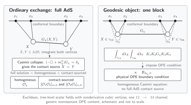
In one Euclidean $12\to34$ channel at tree level, for nonderivative scalar cubic vertices and generic nonresonant dimensions—meaning the relevant Casimir eigenvalues are distinct—the ordinary exchange integrates $X$ and $Y$ over all of AdS; the Green-function source makes its Casimir equation inhomogeneous and its OPE content includes $\mathcal O_\chi$, $[\mathcal O_1\mathcal O_2]_{m,0}$, and $[\mathcal O_3\mathcal O_4]_{n,0}$. Restricting the vertices to $\gamma_{12}$ and $\gamma_{34}$ gives the geodesic object proportional to the physical $(\Delta_\chi,0)$ block after the OPE boundary condition is imposed. Schematic, not to scale, and not a complete crossing-symmetric correlator.

Object	Vertex domain	Casimir status	Generic nonresonant direct-channel content
Ordinary scalar exchange	$X,Y$ range over AdS	Contact-sourced	$\mathcal O_\chi$ plus the two scalar double-trace towers
Geodesic Witten object	$X\in\gamma_{12}$ and $Y\in\gamma_{34}$	Homogeneous; the OPE condition selects the physical branch	One physical $(\Delta_\chi,0)$ block
Zero-derivative $D_{1234}$ contact diagram	One bulk vertex	Source in the displayed exchange equation	Scalar double-trace families; no generic single-trace exchange-pole family

The same relationships are available as a structured figure description.

Single- and double-trace content in the 12→34 channel

For generic external dimensions with the relevant Casimir eigenvalues distinct, and for the nonderivative scalar vertices used here, the direct-channel decomposition is

$$\begin{aligned} \mathcal E_s(x_i)={}&A_\chi\mathcal B_{\Delta_\chi,0}(x_i)\\ &+\sum_{m=0}^{\infty}A_m^{(12)} \mathcal B_{\Delta_1+\Delta_2+2m,0}(x_i)\\ &+\sum_{n=0}^{\infty}A_n^{(34)} \mathcal B_{\Delta_3+\Delta_4+2n,0}(x_i). \end{aligned}$$

There are two scalar double-trace towers. The first is built from the $12$ pair, and the second from the $34$ pair. An unrestricted spin sum would be wrong for this specific zero-derivative scalar construction; more general vertices require a separate decomposition. Hijano and collaborators derive the three displayed terms directly in Hijano et al. 2016, § 4.3, eqs. (4.13)–(4.17), pp. 31–32.

At leading large $N$,

$$[\mathcal O_i\mathcal O_j]_{m,0} \sim \mathcal O_i\Box^m\mathcal O_j+\text{primary completion}, \qquad \Delta_{ij,m}^{(0)}=\Delta_i+\Delta_j+2m.$$

At finite $N$, operator identities and mixing can blur this semiclassical one-particle/two-particle labeling, so the displayed names organize sectors rather than assert a literal trace count.

A coefficient check from the contact source

Suppose the zero-derivative contact diagram has the block decomposition

$$D_{1234}= \sum_m d_m^{(12)}\mathcal B_{\Delta_1+\Delta_2+2m,0} +\sum_n d_n^{(34)}\mathcal B_{\Delta_3+\Delta_4+2n,0}.$$

Project the inhomogeneous Casimir equation onto each nondegenerate block. Since $\mathcal C_{12}\mathcal B_{\Delta,0}=C_{\Delta,0}\mathcal B_{\Delta,0}$ with $C_{\Delta,0}=\Delta(\Delta-d)$,

$$\boxed{ \begin{aligned} A_m^{(12)}&= \frac{\lambda L^2d_m^{(12)}}{C_\chi-C_{\Delta_1+\Delta_2+2m,0}},\\ A_n^{(34)}&= \frac{\lambda L^2d_n^{(34)}}{C_\chi-C_{\Delta_3+\Delta_4+2n,0}}. \end{aligned} }$$

The overall sign follows the declared exchange and contact conventions. Hijano et al. write the inverse using $(\Box-m_\chi^2)$ and an independently normalized kernel; after translating those choices, their result confirms the mass-difference pole structure, while the orientation shown here follows the unit Green equation declared above Hijano et al. 2016, eqs. (4.17)–(4.18), pp. 32–33. This gives a practical check: calculate the contact coefficients once, divide $\lambda L^2d_m$ by the corresponding $C_\chi-C_{\Delta,0}$, and compare with a direct exchange integral.

The homogeneous coefficient is instead set by the Green-function boundary condition and three-point normalizations. With unit-normalized boundary operators it factorizes into the normalized boundary OPE coefficients $C_{12\chi}$ and $C_{34\chi}$ as

$$A_\chi=C_{12\chi}C_{34\chi}.$$

This factorization appears directly in Hijano et al. 2016, § 4.3, eq. (4.16), p. 32. Thus an exchange-pole residue fixes this product, not either cubic coupling in isolation, and only after the bulk field and boundary two-point normalizations have been fixed.

Heavy exchange becomes local

For $m_\chi L\gg1$ and external bulk gradients small compared with $m_\chi$, write the Green operator whose position-space kernel is $G_\chi(X,Y)$ as

$$\widehat G_\chi:=(-\Box+m_\chi^2)^{-1} \sim\frac{1}{m_\chi^2}+\frac{\Box}{m_\chi^4} +O\!\left(\frac{\Box^2}{m_\chi^6}\right).$$

Consequently,

$$\mathcal E_s= \frac{\lambda}{m_\chi^2}D_{1234} +\frac{\lambda}{m_\chi^4} \int d\mu_X\,F_{12}(X)\Box F_{34}(X)+\cdots.$$

Substituting the leading term into the Casimir equation gives $-C_\chi(\lambda/m_\chi^2)D_{1234}=-\lambda L^2D_{1234}$, while the $\mathcal C_{12}$ term is subleading. This checks the sign, the power of $L$, the delta normalization, and the EFT statement that a sufficiently heavy exchange reduces to local contact interactions.

Degeneracy, mixing, and OPE logarithms

The preceding sums assume distinct Casimir eigenvalues. The two external towers can collide when

$$\Delta_1+\Delta_2-\Delta_3-\Delta_4\in2\mathbb Z,$$

and a single-trace level can also collide with a double-trace level. Apparent mass denominators then require a regulated limit or diagonalization in the degenerate operator space. In the all-identical case the two external towers coincide; they must not be counted twice as independent operators.

When the relevant residue survives the limiting procedure, two colliding block contributions combine into a derivative block. In the usual large-$N$ normalization,

$$u^{(\tau_0+\gamma/N^2)/2} =u^{\tau_0/2} \left[1+\frac{\gamma}{2N^2}\log u+O(N^{-4})\right].$$

The $\log u$ coefficient therefore carries anomalous-dimension data. The displayed $N^{-2}$ expansion assumes ordinary double-trace anomalous-dimension power counting after same-order mixing has been resolved. An exact single-trace–double-trace degeneracy coupled at order $N^{-1}$ can instead require degenerate perturbation theory and different power counting. An integer relation among dimensions is a warning of a possible collision, not by itself a proof that a logarithm survives: numerator zeros or mixing can cancel an apparent pole. Hijano et al. display the derivative-block limit in Hijano et al. 2016, § 4.4.2, eqs. (4.24)–(4.26), p. 34, while Liu classifies coincident-pole exceptions in Liu 1999, § 2, pp. 12–14.

Contact freedom and what pole data determine

Once the bulk action, boundary conditions, and normalizations are fixed, its exchange diagram is fixed. The “contact ambiguity” appears when one tries to reconstruct that answer from single-trace exchange poles and residues alone. A local quartic vertex may be added without changing that pole family. It does change the separated-point correlator, the double-trace OPE data, and—in resonant sectors—the anomalous-dimension matrix. Higher-derivative local terms change the allowed polynomial completion.

In Mellin space the distinction is especially transparent: exchange produces a meromorphic single-trace pole sequence, whereas a local contact interaction contributes a polynomial whose degree tracks the derivative order Fitzpatrick et al. 2011, §§ 3.1.3–3.2, eqs. (67) and (70), pp. 22–23. Pole data therefore determine neither a unique polynomial completion nor a unique off-shell field basis. Field redefinitions can reshuffle exchange and contact representatives while leaving the full correlator and factorization residues unchanged Liu 1999, § 3, eqs. (3.1)–(3.7), pp. 14–15.

This contact freedom is different from the block-versus-shadow ambiguity. The latter is a homogeneous Casimir freedom removed by the OPE and bulk boundary conditions; a contact addition changes the inhomogeneous problem itself.

One channel is not a crossing solution

A lone physical block fails the contact-sourced Casimir equation. A lone $s$-channel exchange diagram passes that equation but is still generally not a complete crossing-symmetric four-point function. For identical scalars, a physical tree-level correlator normally combines the allowed $s$-, $t$-, and $u$-channel exchanges with contact terms whose coefficients are fixed by the chosen bulk EFT and crossing constraints.

A geodesic Witten object and an ordinary exchange Witten diagram are therefore distinct:

• the geodesic object isolates one physical conformal family after its boundary condition is chosen;
• the ordinary exchange integrates the vertices over all of AdS and contains the two double-trace towers.

The result established here is limited to a Euclidean tree-level scalar correlator contribution in one channel of a fixed bulk EFT. It is not a flat-space amplitude, a loop result, a proof of a unique bulk Lagrangian, or a complete nonperturbative CFT four-point function.

Common pitfalls

Equating “one internal line” with “one block.” The internal line identifies the single-trace pole family, but integrating its endpoints over all of AdS also creates the contact source and double-trace data.

Calling a contact diagram a boundary contact term. A local bulk vertex gives a nontrivial correlator at separated boundary points. “Contact” describes the number of bulk vertices, not support only at coincident boundary insertions.

Using the generic sums at a resonance. Coincident towers require a limiting calculation and often an operator-mixing problem. Substituting equal dimensions directly into the nondegenerate denominators can manufacture divergences or double count a family.

Testing crossing on one channel. The exact Casimir-source test distinguishes one block from one exchange contribution. Crossing is a separate condition on the channel-summed correlator.

Exercises

1. Derive the contact-sourced equation. Starting from $\mathcal E_s$, use $\mathcal C_{12}F_{12}=L^2\Box F_{12}$ and the declared Green equation to derive the boxed inhomogeneous Casimir equation. Identify the origin of its minus sign.

Solution

Self-adjointness of $\Box$ in the initial convergence domain gives

$$\mathcal C_{12}\mathcal E_s =\lambda L^2\int d\mu_Xd\mu_Y\, F_{12}(X)(\Box_XG_\chi)F_{34}(Y).$$

Because $(-\Box_X+m_\chi^2)G_\chi=\delta_g$,

$$\Box_XG_\chi=m_\chi^2G_\chi-\delta_g.$$

Multiplication by the outer $L^2$ turns the mass term into $m_\chi^2L^2\mathcal E_s=C_\chi\mathcal E_s$. The delta function sets $X=Y$ and gives $D_{1234}$. Therefore

$$(\mathcal C_{12}-C_\chi)\mathcal E_s =-\lambda L^2D_{1234}.$$

The minus sign comes from solving the declared Euclidean kinetic equation for $\Box G_\chi$. A convention that reverses the Green or Casimir sign reverses both sides consistently.

2. Recover both double-trace towers. Assume the displayed contact decomposition with coefficients $d_m^{(12)}$ and $d_n^{(34)}$. Solve the Casimir equation block by block. What changes (a) when $\mathcal O_1=\mathcal O_3=\mathcal O_A$ and $\mathcal O_2=\mathcal O_4=\mathcal O_B$, and (b) when only $\Delta_1=\Delta_3$ and $\Delta_2=\Delta_4$ while the species remain distinct?

Solution

Every physical block is a Casimir eigenfunction, so its exchange coefficient is the corresponding contact coefficient divided by $C_\chi-C_{\Delta,0}$. This gives the two boxed coefficient formulas above and leaves one homogeneous $\Delta_\chi$ block. The nonderivative scalar source contains only spin-zero blocks in this direct-channel decomposition.

In case (a), both sums refer to the same $[\mathcal O_A\mathcal O_B]_{m,0}$ operators. Combine their coefficients before taking the regulated limit; treating them as two independent copies double counts the spectrum. In case (b), equality of dimensions makes the Casimir eigenvalues degenerate but does not identify the operators. The distinct double-trace species remain independent until the interaction-induced mixing matrix is diagonalized.

3. Extract an OPE logarithm. Let a leading block contribution contain $a=a_0+a_1/N^2$ and twist $\tau=\tau_0+\gamma/N^2$. Expand its leading OPE power through order $N^{-2}$.

Solution

Use $u^{\gamma/(2N^2)}=1+\gamma\log u/(2N^2)+O(N^{-4})$:

$$a\,u^{\tau/2} =u^{\tau_0/2} \left[ a_0+\frac{1}{N^2} \left(a_1+\frac{a_0\gamma}{2}\log u\right) \right]+O(N^{-4}).$$

The logarithm measures the anomalous-dimension contribution only after any degenerate operator mixing has been diagonalized.

4. Separate the three completeness tests. Compare (i) one $\mathcal B_{\Delta_\chi,0}$, (ii) one $s$-channel exchange $\mathcal E_s$, and (iii) $\mathcal E_s+\mathcal E_t+\mathcal E_u+\mathcal E_{\mathrm{contact}}$ for identical external scalars. Which equation or requirement tests each object?

Solution

The single block passes the homogeneous Casimir equation but fails the exchange diagram’s nonzero contact-source test. The $s$-channel exchange passes the inhomogeneous $12\to34$ Casimir equation but need not be invariant under permutations of the identical external operators. The channel sum plus allowed contact terms is the candidate crossing-symmetric tree-level correlator; it must still use one normalization, one boundary condition, and one consistent EFT truncation and power counting across all channels. Passing crossing does not make it a loop or nonperturbative answer.

Continue the calculation

• Review the source term: Contact Witten diagrams develops the local bulk integral.
• Understand exchange/contact reshuffling: Bulk field redefinitions and contact ambiguities separates invariant correlator data from off-shell representatives.
• Generalize the internal line: Spinning and tensor Witten diagrams adds tensor structures and gauge constraints.
• Translate to pole language: Mellin contact polynomials and exchange poles separates meromorphic exchange data from polynomial contact freedom.
• Extract the induced spectrum: Double-trace data and large-spin anomalous dimensions continues from a diagram to CFT data.

The chapter overview contains the structure diagram and validity and failure diagram. They are embedded there once so that their shared chapter-level context is not repeated on every article.

For the chapter-wide comparison of assumptions, counterevidence, falsifiers, and claim ceilings, see the claim-domain table.

References

• D’Hoker, Eric, and Daniel Z. Freedman. “Supersymmetric Gauge Theories and the AdS/CFT Correspondence.” In Strings, Branes and Extra Dimensions: TASI 2001, edited by Steven S. Gubser and Jonathan D. Lykken, 3–158. Singapore: World Scientific, 2004. DOI; Open PDF.
• Fitzpatrick, A. Liam, Jared Kaplan, João Penedones, Suvrat Raju, and Balt C. van Rees. “A Natural Language for AdS/CFT Correlators.” Journal of High Energy Physics 2011, no. 11 (2011): 095. DOI; Open PDF.
• Hijano, Eliot, Per Kraus, Eric Perlmutter, and River Snively. “Witten Diagrams Revisited: The AdS Geometry of Conformal Blocks.” Journal of High Energy Physics 2016, no. 1 (2016): 146. DOI; Open PDF.
• Liu, Hong. “Scattering in Anti-de Sitter Space and Operator Product Expansion.” Physical Review D 60 (1999): 106005. DOI; Open PDF.