Quantum-Cosmology Observables and the Problem of Time

In a constrained cosmology, a prediction is not $|\Psi(q)|^2$. It is a probability or expectation value for a Dirac or relational observable in a specified physical state and positive physical inner product, conditioned on a valid clock reading or assigned to a decoherent history. This page makes those data explicit and tests them in a solvable massless-scalar minisuperspace. It does not select a unique clock, state, factor ordering, or solution of the problem of time in full general relativity.

Required background. Wheeler–DeWitt Quantization and the Problem of Time supplies constraint quantization. Relational and Gauge-Invariant Gravitational Observables supplies the observable standard.

Helpful background. Constraint Solving and the Observable Dictionary and Relativistic Protocols, Clocks, Encoding, and Channel Tomography supply gauge and protocol checks.

From a constraint solution to a prediction

A kinematical wavefunction lives before all constraints and gauge redundancies have been removed. A physical state instead solves the declared constraints and belongs to a physical Hilbert space with a positive product. An observable must act on that space and preserve the constraint; in a generally covariant theory it often answers a relational question such as “what is the value of $A$ when the clock $T$ reads $\tau$?” Complete observables make that question into a family of Dirac observables Rovelli 1991, §§II–III; Dittrich 2006, §§2–4. Kiefer and Peter 2022, §§2–5 review how this problem appears in quantum cosmology.

The minimum prediction contract is therefore:

Data required before a quantum-cosmology probability is meaningful

Required datum	Question it answers	Failure if omitted
Configuration space and constraints	Which variables, gauge generators, truncations, and domains define the model?	A formal solution may still contain gauge redundancy or solve a different operator equation.
Physical state and state-selection data	Which constraint solution, boundary condition, frequency sector, and branch are used?	The dynamics does not select an initial or boundary state by itself.
Positive physical product and measure	How are states normalized, and with respect to which measure?	A conserved indefinite current or a bare modulus squared is not a Born probability.
Relational observable	Which physical quantity is evaluated at which clock reading or conditioning event?	A bare scale factor is gauge dependent; the conditioned scale factor can be physical on a clock patch.
Clock domain and resolution	Where is the clock monotonic, transverse to the gauge flow, and sufficiently sharp?	Multiple intersections, turning points, or broad clock states make the answer branch or resolution dependent.
Records, alternatives, and decoherence	Which mutually exclusive alternatives are assigned probabilities, and what records distinguish them?	Interfering multi-time histories need not obey probability sum rules.
Approximation and claim boundary	Which inhomogeneous modes, backreaction terms, and full-theory constraints were discarded?	An exact minisuperspace answer can be mistaken for an exact prediction of quantum gravity.

Group averaging, relational Dirac observables, Page–Wootters conditioning, and reduced Schrödinger evolution can agree when the reduction maps, frequency sector, clock observable, and physical product are matched. The equivalence is a construction with hypotheses, not a license to move between clocks informally Höhn, Smith, and Lock 2021, §§2 and 5–7.

A solvable scalar-clock universe

Consider a spatially flat FLRW metric with a homogeneous massless scalar. This is a finite-dimensional specialization of the canonical constraint problem introduced by DeWitt 1967, §4:

$$ds^2=N^2dt^2-a^2(t)d\mathbf x^2,$$

and regulate the noncompact spatial integral with a fixed comoving cell of coordinate volume $V_0$. With reduced Planck mass $M_{\mathrm{Pl}}=(8\pi G)^{-1/2}$ and $c=\hbar=1$, the reduced Lagrangian is

$$L=V_0\left(-\frac{3M_{\mathrm{Pl}}^2a\dot a^2}{N} +\frac{a^3\dot\phi^2}{2N}\right).$$

Its momenta and Hamiltonian constraint are

$$\begin{aligned} p_a&=-\frac{6V_0M_{\mathrm{Pl}}^2a\dot a}{N}, &p_\phi&=\frac{V_0a^3\dot\phi}{N},\\ \mathcal C&=-\frac{p_a^2}{12V_0M_{\mathrm{Pl}}^2a} +\frac{p_\phi^2}{2V_0a^3}\approx0. \end{aligned}$$

Define the dimensionless variables

$$\alpha=\ln\frac{a}{a_\star}, \qquad \varphi=\frac{\phi}{\sqrt6M_{\mathrm{Pl}}}, \qquad p_\alpha=ap_a, \qquad p_\varphi=\sqrt6M_{\mathrm{Pl}}p_\phi.$$

Multiplication by the positive function $12V_0M_{\mathrm{Pl}}^2a^3$ gives the classically equivalent densitized constraint

$$\mathcal C_0=p_\varphi^2-p_\alpha^2\approx0.$$

This step is harmless classically for $a>0$ but is part of the quantization choice: densitizing before quantization can change the measure, ordering, and self-adjointness problem. The model is exact only after that choice and the homogeneous truncation have been declared. Closely related flat-FLRW scalar-clock models and their clock-dependent domains are analyzed in Gielen and Menéndez-Pidal 2022, §§2–5.

Use the auxiliary representation $L^2(\mathbb R^2,d\alpha\,d\varphi)$ with $p_\alpha=-i\partial_\alpha$ and $p_\varphi=-i\partial_\varphi$, and choose the symmetric spatial realization

$$\widehat\Theta=-\frac{d^2}{d\alpha^2}, \qquad D(\widehat\Theta)=H^2(\mathbb R), \qquad \mathcal H_\alpha=L^2(\mathbb R,d\alpha).$$

It is non-negative and self-adjoint, so the spectral theorem defines

$$\widehat H=\sqrt{\widehat\Theta}=|\widehat p_\alpha|, \qquad D(\widehat H)=H^1(\mathbb R).$$

Because $\alpha$ covers the full real line, the endpoints $a=0$ and $a=\infty$ lie at $\alpha=-\infty$ and $\alpha=+\infty$; this realization has no additional finite-endpoint self-adjoint-extension parameter.

The Wheeler–DeWitt equation is the $1+1$ dimensional wave equation

$$(\partial_\varphi^2-\partial_\alpha^2)\Psi(\alpha,\varphi)=0.$$

We now make two state-space choices rather than hiding them. First select the positive-$p_\varphi$ sector,

$$-i\partial_\varphi\Psi=\widehat H\Psi, \qquad U(\Delta\varphi)=e^{+i\widehat H\Delta\varphi}.$$

Second select its expanding chiral branch, for which $p_\alpha<0$. In the Newton–Wigner-normalized frequency-sector representation obtained from the group-averaged product, the physical product is

$$\langle\Psi_1|\Psi_2\rangle_{\mathrm{phys}} =\int_{-\infty}^{\infty}d\alpha\, \Psi_1^*(\alpha,\varphi_0)\Psi_2(\alpha,\varphi_0),$$

independent of the representative slice $\varphi_0$. After the frequency-dependent spectral weight is absorbed into $A(k)$, the amplitude has the equivalent $L^2$ product in $k$. This is the declared positive physical product after frequency reduction; it is not the unprocessed, indefinite Klein–Gordon current. The corresponding group-averaged product, frequency split, and single-clock-time projectors in the flat-FLRW scalar model are developed by Craig and Singh 2010, §§III.B and V.A.1. The distinction between conserved and positive products is essential in quantum cosmology Gielen and Menéndez-Pidal 2022, §3.1.

The relational scale factor

Let $E_\Delta$ multiply by the indicator of an interval $\Delta\subset\mathbb R$ in $\alpha$. At clock reading $\varphi=\tau$, its physical representative on the reference slice $\varphi_0$ is

$$E_{\Delta|\tau}^{(\varphi_0)} =U(\tau-\varphi_0)^\dagger E_\Delta U(\tau-\varphi_0).$$

This family is the reduced-model complete observable “$\alpha$ lies in $\Delta$ when the scalar reads $\tau$.” It is not the bare scale factor and not a complete four-dimensional diffeomorphism-invariant observable. In the declared physical representation,

$$\Pr(\alpha\in\Delta\mid\varphi=\tau) =\langle\Psi(\varphi_0)|E_{\Delta|\tau}^{(\varphi_0)}|\Psi(\varphi_0)\rangle_{\mathrm{phys}} =\int_\Delta d\alpha\,|\Psi(\alpha,\tau)|^2.$$

The second equality is special to this deparametrized, one-frequency model with the stated clock and product. It is not a generic rule that $|\Psi|^2$ on superspace is a probability.

An exactly normalized expanding packet

For $k>0$, choose

$$A_\kappa(k) =\frac{k^2e^{-k/(2\kappa)}e^{ik\alpha_0}} {\sqrt{24\kappa^5}}, \qquad A_\kappa(k)=0\quad\text{for }k\le0.$$

The branch restriction is exact, not a Gaussian-tail approximation, and

$$\int_0^\infty dk\,|A_\kappa(k)|^2 =\frac{1}{24\kappa^5}\int_0^\infty dk\,k^4e^{-k/\kappa}=1.$$

Evolution gives

$$\begin{aligned} \Psi_\kappa(\alpha,\varphi) &=\frac{1}{\sqrt{2\pi}} \int_0^\infty dk\,A_\kappa(k)e^{-ik\alpha+ik\varphi}\\ &=\frac{1}{\sqrt{12\pi\kappa^5}} \left[\frac{1}{2\kappa}+i(\alpha-\alpha_0-\varphi)\right]^{-3}. \end{aligned}$$

Therefore

$$\rho_\alpha(\alpha\mid\varphi) =\frac{1}{12\pi\kappa^5} \left[\frac{1}{4\kappa^2} +(\alpha-\alpha_0-\varphi)^2\right]^{-3}.$$

Take the reproducible fixture $\kappa=1/2$ and $\alpha_0=0$. Then

$$\rho_\alpha(\alpha\mid\varphi) =\frac{8}{3\pi}\frac{1}{[1+(\alpha-\varphi)^2]^3}, \qquad \langle\alpha\rangle_\varphi=\varphi, \qquad (\Delta\alpha)^2=\frac13.$$

The probability of lying within one unit of the packet center is

$$\Pr(|\alpha-\varphi|\le1\mid\varphi) =\frac12+\frac{4}{3\pi} =0.924413181578\ldots.$$

Because $d\alpha=da/a$, the density with respect to $da$ is

$$p_a(a\mid\varphi) =\frac{1}{a}\, \rho_\alpha\!\left(\ln\frac{a}{a_\star}\,\middle|\,\varphi\right),$$

and the same event is

$$e^{\varphi-1}\le\frac{a}{a_\star}\le e^{\varphi+1}.$$

The zero of $\alpha$ and the fiducial scale $a_\star$ are conventional; changes $\Delta\alpha$ are the useful relational quantity. The packet has polynomial tails, so bounded interval probabilities and the displayed log-scale moments are well defined, but positive moments of the unbounded operator $a=a_\star e^\alpha$ diverge. We do not quote $\langle a\rangle$.

Rematch the clock, not just its label

The upper panel below displays the probability just calculated. The lower panel performs a positive clock-relabeling control and a deliberate failure. Define $\tau=2\varphi$. The chain rule requires

$$-i\partial_\tau\Psi=\frac{\widehat H}{2}\Psi.$$

At the same physical event $s=\varphi=\tau/2$, the correctly rematched $\tau$ description has exactly the same density, norm, and mean as the $\varphi$ description. If one changes the clock label but incorrectly keeps $\widehat H_\tau=\widehat H$, the state remains normalized while its mean becomes $2s$. At $s=2$, the correct and incorrect centers are $2$ and $4$, and their total-variation distance is

$$d_{\mathrm{TV}} =\frac12\int d\alpha\, |\rho_{\mathrm{correct}}-\rho_{\mathrm{naive}}| =\frac12+\frac{4}{3\pi} =0.924413181578\ldots.$$

Norm conservation alone therefore does not establish clock equivalence.

On a narrow screen, swipe or use the Left and Right arrow keys to pan across the figure. Home and End move to its edges. A full-size link is also available.

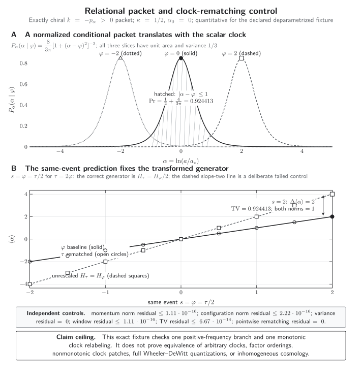
Relational packet and clock-rematching control for the exact $\kappa=1/2$ fixture. Panel A shows $\rho_\alpha(\alpha\mid\varphi)$ at $\varphi=-2,0,2$; each curve has unit area, variance $1/3$, and unchanged shape. Panel B compares the same-event coordinate $s=\varphi=\tau/2$. The correctly transformed generator $H_\tau=H_\varphi/2$ coincides with the baseline, whereas the dashed, deliberately unrescaled generator preserves normalization but produces slope two. At $s=2$ its center is displaced from $2$ to $4$, giving $d_{\mathrm{TV}}=0.924413\ldots$. The curves are quantitative for the stated equations and are not evidence for a preferred cosmological clock.

Open the full-size SVG, download the plotted CSV data, or inspect the complete semantic record.

Numerical relationships encoded by the two-panel clock-control figure

Series or control	Clock or event label	Generator	Norm	Mean log scale	Variance	Probability within one unit of that curve’s mean	Total-variation distance from the same-event ϕ baseline	Status
Baseline packet	Scalar clock ϕ = −2	Hϕ	1	−2	1/3	0.924413181578…	0 against itself	Exact analytic fixture
Baseline packet	Scalar clock ϕ = 0	Hϕ	1	0	1/3	0.924413181578…	0 against itself	Exact analytic fixture
Baseline packet	Scalar clock ϕ = 2	Hϕ	1	2	1/3	0.924413181578…	0 against itself	Same-event reference at s = 2
Correct τ rematching	τ = 4 and s = τ/2 = 2	Hτ = Hϕ/2	1	2	1/3	0.924413181578…	0	Exact pointwise rematching
Naive unrescaled generator	τ = 4 and s = 2	Deliberately wrong Hτ = Hϕ	1	4	1/3	0.924413181578…	0.924413181578…	Failed same-event control

The same physical projector is also independent of the reference slice used to represent it. If $\varphi_1$ replaces $\varphi_0$, rematch the state by

$$|\Psi(\varphi_1)\rangle =U(\varphi_1-\varphi_0)|\Psi(\varphi_0)\rangle.$$

The group law then gives

$$\begin{aligned} &\langle\Psi(\varphi_1)|E_{\Delta|\tau}^{(\varphi_1)}|\Psi(\varphi_1)\rangle\\ &\qquad= \langle\Psi(\varphi_0)|E_{\Delta|\tau}^{(\varphi_0)}|\Psi(\varphi_0)\rangle. \end{aligned}$$

This exact equality tests a change of representation surface, not a change of physical clock.

A clock that loses its patch

Now choose the nonlinear candidate $\chi=\varphi^2$. It is not a global clock. Its transversality factor is

$$\{\chi,\mathcal C_0\}=4\varphi p_\varphi,$$

which vanishes at $\varphi=0$. Moreover, $\chi=4$ intersects the same expanding family at both $\varphi=+2$ and $\varphi=-2$. Conditioning only on $\chi=4$ therefore does not specify a unique relational observable.

For example, imposing an equal-weight, branch-blind rule produces

$$\rho_{\mathrm{mix}}(\alpha\mid\chi=4) =\frac12\rho_\alpha(\alpha\mid\varphi=2) +\frac12\rho_\alpha(\alpha\mid\varphi=-2),$$

with

$$\langle\alpha\rangle_{\mathrm{mix}}=0, \qquad (\Delta\alpha)^2_{\mathrm{mix}}=\frac{13}{3}.$$

The mixture is normalized, but neither the constraint nor the clock reading supplies the equal weights. It is not equivalent to either branch. The exact downgrade cause is the loss of a one-to-one clock patch; an added branch label or a new clock is required. Clock changes in quantum theory must transform states, observables, and products through a common physical description on their overlap Höhn and Vanrietvelde 2020, §§2–4.

Finite clock resolution

An ideal clock slice is also an approximation. Let $w_\sigma(\varphi-\tau)\ge0$ be a normalized, symmetric clock-response window with variance $\sigma_\varphi^2$. The finite-resolution probability is

$$P_\sigma(\Delta\mid\tau) =\frac{\displaystyle\int d\varphi\, w_\sigma(\varphi-\tau) \langle\Psi(\varphi)|E_\Delta|\Psi(\varphi)\rangle} {\displaystyle\int d\varphi\, w_\sigma(\varphi-\tau) \langle\Psi(\varphi)|\Psi(\varphi)\rangle}.$$

Unitary evolution makes the denominator one. If the ideal probability $P(\tau)$ is smooth across the window,

$$P_\sigma(\tau) =P(\tau)+\frac{\sigma_\varphi^2}{2}P''(\tau) +O(\mu_4).$$

Thus finite resolution preserves normalization but changes a local interval probability in a controlled way. A fully quantum clock is more than a classical smearing window; Page–Wootters conditioning uses clock-system correlations, and relativistic constraints can require a covariant clock POVM rather than a self-adjoint time operator Page and Wootters 1983; Höhn, Smith, and Lock 2021, §§3–6.

Records and decoherent histories

The single-clock-time alternatives $E_\Delta$ and $1-E_\Delta$ are orthogonal projectors, so their Born probabilities add on the declared slice. A question such as “did the universe ever enter region $\Delta$?” is different: it concerns an entire history, not one relational instant.

For coarse-grained histories $h$, constraint-compatible class operators $C_h$ define the decoherence functional

$$D(h,h') =\langle\Psi|C_{h'}^\dagger C_h|\Psi\rangle_{\mathrm{phys}}.$$

Only when the off-diagonal terms are negligible at a stated tolerance may one assign additive probabilities $p(h)=D(h,h)$. Internal records—correlations in other degrees of freedom—can support that interpretation even though there is no external observer. Decoherence does not create the physical inner product, choose the state, or cure a bad clock. Halliwell constructs constraint-commuting class operators for entering regions of minisuperspace and shows where the semiclassical approximation and decoherence enter Halliwell 2009, §§I.C and III–VI.

What survives the tests

Controls, failures, and the strongest licensed conclusion

Test	Result	Interpretation
Packet normalization	Pass. The spectral and configuration-space norms are exactly one.	A positive single-time probability exists in the declared physical product.
Reference-slice change	Pass. State and projector rematching gives exact equality.	The answer does not depend on the slice used to represent the same relational observable.
Clock relabeling	Pass only with chain-rule rematching. The correct total-variation residual is zero.	Relabeling a clock is harmless only when the generator and event label transform together.
Unrescaled generator	Fail. The norm stays one, but the benchmark gives total-variation distance 0.924413…	Unitarity is necessary, not sufficient, for clock equivalence.
Nonmonotonic clock	Fail globally. The conditioning surface is tangent at zero and double-valued at χ = 4.	Branch weights are extra physical data; restrict to a patch or change clocks.
Different ordering or full theory	Not established. The chosen densitization, measure, domain, sector, and homogeneous truncation remain fixed.	No ordering-independent or full-quantum-gravity prediction follows.

The strongest surviving claim is precise: within the fixed positive-$p_\varphi$, expanding, symmetric-ordering quantization, normalized single-clock-time log-scale probabilities are independent of the fiducial representation slice and of a harmless clock relabeling when every object is rematched. The calculation does not establish a global clock, unique state, unique factor ordering, multi-time decoherence, control of inhomogeneous modes, or a prediction of full quantum gravity. Explicit models with more degrees of freedom show that demanding unitarity relative to different clocks can lead to different domains and qualitatively different cosmological behavior Gielen and Menéndez-Pidal 2022, §§3–6; Bojowald and Halnon 2018.

Common pitfalls

Treating $|\Psi|^2$ as a superspace probability. The measure and positive physical product must first be specified. The packet above has a Born density only after frequency reduction and the $L^2(d\alpha)$ product have been declared.

Equating a frozen constraint with absence of change. The gauge parameter generated by the constraint is not an external time. Relational observables can change with one physical variable relative to another.

Calling the bare scale factor an observable. The page computes the family “$\alpha$ when $\varphi=\tau$.” It does not promote the kinematical $a$ at an arbitrary coordinate time to a Dirac observable.

Assuming positive frequency is forced by the constraint. The quadratic constraint has two frequency sectors, and this page chooses one plus an expanding chiral branch. Reversing the scalar orientation is a different but related sector choice.

Confusing normalization with clock equivalence. Both the correct and deliberately incorrect $\tau$ evolutions preserve norm. Only the rematched generator reproduces the same event probabilities.

Letting decoherence do too much. Decoherence licenses probability sum rules for a declared coarse graining. It does not select the state, define the physical product, or prove that a minisuperspace truncation approximates the full theory.

Exercises

1. Derive the densitized constraint

Starting from the reduced Lagrangian, derive $p_a$, $p_\phi$, the Hamiltonian constraint, and $\mathcal C_0=p_\varphi^2-p_\alpha^2$.

Solution

Differentiation with respect to the velocities gives

$$p_a=-\frac{6V_0M_{\mathrm{Pl}}^2a\dot a}{N}, \qquad p_\phi=\frac{V_0a^3\dot\phi}{N}.$$

Solving for the velocities and forming $p_a\dot a+p_\phi\dot\phi-L$ yields

$$H=N\left(-\frac{p_a^2}{12V_0M_{\mathrm{Pl}}^2a} +\frac{p_\phi^2}{2V_0a^3}\right).$$

Since $p_\alpha=ap_a$ and $p_\varphi=\sqrt6M_{\mathrm{Pl}}p_\phi$, multiplication by $12V_0M_{\mathrm{Pl}}^2a^3$ gives

$$-p_\alpha^2+p_\varphi^2\approx0.$$

The multiplier is positive only on the chosen $a>0$ sector; its use before quantization is part of the model definition.

2. Check the packet and the scale-factor measure

Verify the spectral normalization, the density for $\kappa=1/2$, its mean and variance, and the probability $\Pr(|\alpha-\varphi|\le1)$. Then transform the density from $\alpha$ to $a$.

Solution

Use

$$\int_0^\infty dk\,k^4e^{-k/\kappa}=4!\,\kappa^5=24\kappa^5$$

and Parseval’s identity. For $y=\alpha-\varphi$ and $\kappa=1/2$,

$$\rho(y)=\frac{8}{3\pi}(1+y^2)^{-3}.$$

Oddness gives $\langle y\rangle=0$, while standard beta-function integrals give $\langle y^2\rangle=1/3$. Direct integration from $-1$ to $1$ gives

$$\int_{-1}^{1}dy\,\rho(y)=\frac12+\frac{4}{3\pi}.$$

Finally $d\alpha=da/a$, so probability conservation requires $p_a(a)=\rho(\ln(a/a_\star))/a$.

3. Rematch two clock descriptions

For $\tau=2\varphi$, derive the correct generator. At the same-event value $s=2$, compute the correct and naive centers and the total-variation distance. Explain why equal norms do not settle the comparison.

Solution

Because $\partial_\tau=\tfrac12\partial_\varphi$,

$$-i\partial_\tau\Psi=\frac{H}{2}\Psi.$$

At $s=\varphi=\tau/2=2$, the correctly rematched density is centered at $2$. Keeping $H$ instead of $H/2$ translates the packet by $\tau=4$. The two equal-shape densities cross at $\alpha=3$, so their total-variation distance is the mass of either density between its center minus one and center plus one:

$$d_{\mathrm{TV}} =\int_{-1}^{1}dy\,\frac{8}{3\pi}(1+y^2)^{-3} =\frac12+\frac{4}{3\pi}.$$

Both generators are self-adjoint and both preserve norm; only one represents the same clock-labeled physical event.

4. Locate the nonlinear-clock failure

Compute the transversality factor, identify the two branches at $\chi=4$, and verify the variance of the equal-weight mixture.

Solution

The Poisson bracket is $\{\chi,\mathcal C_0\}=4\varphi p_\varphi$, so the clock is tangent to the gauge flow at $\varphi=0$. The value $\chi=4$ permits $\varphi=\pm2$. Each component has variance $1/3$ and mean $\pm2$. The law of total variance gives

$$\operatorname{Var}(\alpha) =\frac12\left(\frac13+2^2\right) +\frac12\left(\frac13+(-2)^2\right) =\frac{13}{3}.$$

Choosing equal weights is an additional conditioning rule, not a consequence of $\chi=4$.

5. Resolve a finite-width clock

For a normalized symmetric clock window, expand the finite-resolution probability through second order in the clock width.

Solution

Write $u=\varphi-\tau$ and expand

$$P(\tau+u)=P(\tau)+uP'(\tau)+\frac{u^2}{2}P''(\tau)+\cdots.$$

Normalization gives $\int du\,w_\sigma(u)=1$, symmetry removes the linear term, and the second moment is $\sigma_\varphi^2$. Hence

$$P_\sigma(\tau) =P(\tau)+\frac{\sigma_\varphi^2}{2}P''(\tau)+O(\mu_4).$$

The result quantifies classical response-window uncertainty; a quantum clock can add state-dependent correlations not captured by this convolution.

6. Test history additivity

Let two exclusive coarse histories have class operators $C_1$ and $C_2$. Show exactly how interference obstructs additivity for their union.

Solution

The union has class operator $C=C_1+C_2$, so

$$\begin{aligned} p(1\mathbin{\text{ or }}2) &=\langle\Psi|C^\dagger C|\Psi\rangle\\ &=p(1)+p(2)+2\operatorname{Re}D(1,2). \end{aligned}$$

The ordinary sum rule holds only when the off-diagonal decoherence functional is zero, or negligible compared with a stated tolerance. Orthogonality at one clock slice does not automatically prove decoherence for a multi-time history.

Where to continue

Derive and test the homogeneous truncation before interpreting this exact reduced solution. Then compare Wheeler–DeWitt boundary data, orderings, and inner products and analyze records and semiclassical decoherence.

The chapter structure map places the clock-and-state declaration before approximation and recovery tests. Use the validity map and claim-domain comparison to distinguish this conditional probability from boundary-state, history, bounce, and full singularity-resolution claims.

For the physical-treatment handoff, develop cosmological QFT observables and correlators. For rigorous constraint, measure, and Hilbert-space questions, consult Mathematical QFT. Dated frontier claims and open alternatives belong in the Holography and Quantum Gravity research field.

References

• Bojowald, M., and T. Halnon. “Time in Quantum Cosmology.” Physical Review D 98 (2018): 066001. DOI.
• Craig, D. A., and P. Singh. “Consistent Probabilities in Wheeler–DeWitt Quantum Cosmology.” Physical Review D 82 (2010): 123526. DOI.
• DeWitt, B. S. “Quantum Theory of Gravity. I. The Canonical Theory.” Physical Review 160 (1967): 1113–1148. DOI.
• Dittrich, B. “Partial and Complete Observables for Canonical General Relativity.” Classical and Quantum Gravity 23 (2006): 6155–6184. DOI.
• Gielen, S., and L. Menéndez-Pidal. “Unitarity, Clock Dependence and Quantum Recollapse in Quantum Cosmology.” Classical and Quantum Gravity 39 (2022): 075011. DOI. Open PDF.
• Halliwell, J. J. “Probabilities in Quantum Cosmological Models: A Decoherent Histories Analysis Using a Complex Potential.” Physical Review D 80 (2009): 124032. DOI. Open PDF.
• Höhn, P. A., A. R. H. Smith, and M. P. E. Lock. “Equivalence of Approaches to Relational Quantum Dynamics in Relativistic Settings.” Frontiers in Physics 9 (2021): 587083. DOI.
• Höhn, P. A., and A. Vanrietvelde. “How to Switch between Relational Quantum Clocks.” New Journal of Physics 22 (2020): 123048. DOI.
• Kiefer, C., and P. Peter. “Time in Quantum Cosmology.” Universe 8 (2022): 36. DOI.
• Page, D. N., and W. K. Wootters. “Evolution without Evolution: Dynamics Described by Stationary Observables.” Physical Review D 27 (1983): 2885–2892. DOI.
• Rovelli, C. “Time in Quantum Gravity: An Hypothesis.” Physical Review D 43 (1991): 442–456. DOI.