Lorentzian Einstein–Rosen Bridges and Two-Boundary States

The maximally extended neutral AdS black hole has two exterior regions. A spacelike slice can connect their asymptotic boundaries through an Einstein–Rosen bridge, even though no future-directed causal curve can travel from one boundary to the other. In a controlled semiclassical holographic regime, the standard two-boundary state is the thermofield double (TFD) of two noninteracting boundary theories.

Three qualifications are essential. The TFD and its thermal marginals are exact Hilbert-space statements, whereas the smooth eternal geometry requires a dominant, weakly curved bulk saddle. Boundary times select a relationally anchored bridge slice; the slice and its regulated volume are not intrinsic, slicing-independent sizes of a wormhole. Finally, one-sided thermal density matrices do not determine the purification, its cross-boundary correlations, or a unique interior.

Required background. Two-Sided Black Holes and Thermofield-Double States supplies the thermal state preparation. Relational, Boundary, and Asymptotic Observables supplies the observable standard.

Helpful background. Reflected Entropy and Canonical Purifications gives a purification comparison. Relational Bulk Observables and Dressing Choices explains why gravitational localization requires dressing.

From a simple horizon to four Kruskal regions

Use the site convention $(+---)$ and restrict the construction to a neutral, nonrotating, nonextremal Schwarzschild–AdS-like solution,

$$ds^2=f(r)dt^2-\frac{dr^2}{f(r)}-r^2d\Sigma_{d-1}^2, \qquad f(r)=k+\frac{r^2}{L^2}-\frac{\mu}{r^{d-2}}.$$

Here $d\Sigma_{d-1}^2$ has normalized curvature $k=1,0,$ or $-1$. Let $r_h$ be the largest simple root,

$$f(r_h)=0, \qquad f'(r_h)=2\kappa>0, \qquad \beta=\frac{2\pi}{\kappa}=\frac{4\pi}{f'(r_h)}.$$

The ordinary $(t,r)$ chart fails at $r=r_h$, but the geometry need not. Define the tortoise and null coordinates

$$r_*(r)=\int^r\frac{dr'}{f(r')}, \qquad u=t-r_*, \qquad v=t+r_*.$$

Near a simple horizon,

$$f(r)=2\kappa(r-r_h)+O\!\left((r-r_h)^2\right), \qquad r_*=\frac{1}{2\kappa}\log\lvert r-r_h\rvert+O(1).$$

In the right exterior choose

$$U=-e^{-\kappa u}, \qquad V=e^{\kappa v}.$$

Then $UV=-e^{2\kappa r_*}\propto-(r-r_h)$, and the radial metric becomes

$$ds^2_{(2)}=-\frac{f(r)}{\kappa^2UV}\,dU\,dV.$$

Because $f/(UV)$ has a finite nonzero horizon limit, $U=0$ and $V=0$ are regular null horizons rather than curvature singularities. Analytic continuation gives four sign regions:

Region	Signs	Interpretation
Right exterior $I_R$	$U<0$, $V>0$	Right asymptotic boundary and exterior
Left exterior $I_L$	$U>0$, $V<0$	Left asymptotic boundary and exterior
Future region $II$	$U>0$, $V>0$	Black-hole interior ending at the future singularity
Past region $IV$	$U<0$, $V<0$	White-hole interior beginning at the past singularity

The bifurcation surface $B$ is the codimension-two surface $U=V=0$. Compact coordinates such as $\mathcal U=\arctan U$ and $\mathcal V=\arctan V$ place infinity at finite coordinate distance while preserving null directions. This produces the Penrose diagram below. The conformal drawing is schematic, but the incidences—two timelike boundaries, four horizon branches, two spacelike singularities, and four regions—are causal data Maldacena 2003, § 2, Figures 1–3 and eqs. (2.1)–(2.6).

The stationary Killing field is

$$\xi=\partial_t =\kappa\!\left(V\partial_V-U\partial_U\right).$$

Let $t_L$ and $t_R$ both increase toward the physical future of their respective boundary theories. The same bulk vector then has opposite orientation in the exteriors,

$$\left.\xi\right|_{I_R}=+\partial_{t_R}, \qquad \left.\xi\right|_{I_L}=-\partial_{t_L}.$$

It becomes spacelike behind the horizons. This sign reversal is the source of the two different Hamiltonian combinations below; it is not a convention that can be silently dropped.

The bridge is codimension-one spatial connectivity on a chosen spacelike slice. By contrast, $B$ is codimension two and is minimal on the reflection-symmetric slice. No future-directed causal curve connects the two conformal boundaries: after crossing either future event horizon, such a curve terminates at the future spacelike singularity instead of emerging through the opposite exterior. “Spacelike connected” therefore does not mean “causally connected.”

The thermofield double fixes the clock convention

The prerequisite page develops the Euclidean half-circle preparation and thermal trace in detail. Here only the state identity needed for the Lorentzian geometry is recalled. Let $\Theta$ be the antiunitary map that identifies the two copies and write $\lvert\bar n\rangle_L=\Theta\lvert n\rangle_R$. For matched spectra,

$$\lvert\mathrm{TFD}_\beta\rangle =\frac{1}{\sqrt{Z(\beta)}} \sum_n e^{-\beta E_n/2}\lvert\bar n\rangle_L\lvert n\rangle_R, \qquad \rho_L=\rho_R=\frac{e^{-\beta H}}{Z(\beta)}.$$

Both reduced density matrices are exactly thermal, and

$$(H_R-H_L)\lvert\mathrm{TFD}_\beta\rangle=0.$$

Time evolution with both physical boundary clocks future-directed gives

$$\begin{aligned} \lvert\mathrm{TFD};t_L,t_R\rangle &=e^{-i(H_Lt_L+H_Rt_R)}\lvert\mathrm{TFD}_\beta\rangle \\ &=\frac{1}{\sqrt Z}\sum_n e^{-\beta E_n/2-iE_n(t_L+t_R)} \lvert\bar n\rangle_L\lvert n\rangle_R . \end{aligned}$$

Thus the state depends on

$$\tau\equiv t_L+t_R,$$

whereas the shift $(t_L,t_R)\mapsto(t_L-s,t_R+s)$ is generated by $H_R-H_L$ and leaves both $\tau$ and the TFD unchanged. The figure makes this distinction visible. Inspect the two boundary-time arrows separately from the dashed Killing arrows, and compare the unarrowed spacelike slices with the causal curve that ends at the singularity.

On a narrow screen, swipe or use the Left and Right arrow keys to pan across the figure. Home and End move to its edges. A full-size link is also available.

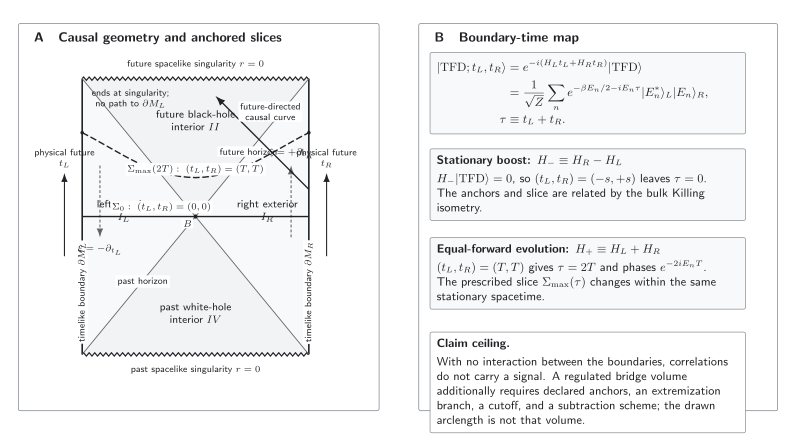
Schematic radial Penrose diagram of a nonextremal, uncharged, nonrotating eternal AdS black hole, with angular directions suppressed. Both physical boundary times increase toward the future, while the stationary Killing field satisfies $\xi=\partial_{t_R}=-\partial_{t_L}$. Consequently $H_R-H_L$ leaves the TFD invariant, whereas equal-forward evolution by $H_L+H_R$ changes $\tau=t_L+t_R$ and the maximal spacelike slice anchored at those times. In the uncoupled geometry, a causal curve entering a future horizon ends at the future singularity rather than reaching the opposite boundary. The bridge is slice-dependent spatial connectivity, not a timelike tube; the drawn curve length does not represent $V_{\max}$, which requires a declared extremization and renormalization prescription. Not to scale. Accessible figure data (JSON)

The same content in linear form is:

Evolution	Future-directed anchors	Effect on the TFD	Bulk interpretation	Licensed conclusion
Reference	$(0,0)$	No relative phase	$\Sigma_0$ crosses $B$	Standard nontraversable two-sided saddle, in its controlled regime
Stationary boost $e^{-is(H_R-H_L)}$	$(-s,+s)$	State invariant	Anchors and slice are related by a Killing isometry	No physical bridge-growth inference
Equal-forward $e^{-iT(H_L+H_R)}$	$(T,T)$	Phase $e^{-2iE_nT}$	A different $\Sigma_{\max}(2T)$ in the same stationary spacetime	Its regulated maximal volume may change within the declared prescription
No interboundary coupling	Any anchors	Marginals remain local thermal states	Future causal curves that enter the hole hit the singularity	Correlation does not imply traversability

For a Hermitian, CPT-even scalar, a safe operator convention is

$$O_L(t_L)=\Theta O_R(-t_L)\Theta^{-1}.$$

The opposite-side Wightman function is then

$$\begin{aligned} G_{LR}(t_L,t_R) &=\frac{1}{Z}\operatorname{Tr}\!\left[ e^{-\beta H/2}O_R(-t_L)e^{-\beta H/2}O_R(t_R) \right] \\ &=\frac{1}{Z}\sum_{m,n}e^{-\beta(E_m+E_n)/2} e^{i(E_n-E_m)\tau}\lvert O_{mn}\rvert^2 . \end{aligned}$$

The dependence is on $\tau=t_L+t_R$, as the state calculation requires. Charged, spinning, or CPT-odd operators need their own transpose, dagger, and charge-conjugation conventions; the scalar formula should not be reused blindly.

Boundary anchors define the bridge slice

Fix a radial cutoff $r_c$ and the boundary cross-sections at $(t_L,t_R)$. Among an explicitly stated class of spacelike codimension-one surfaces $\Sigma$ joining those anchors, define

$$V_{\max}(t_L,t_R;r_c) =\operatorname*{max}_{\partial\Sigma=(t_L,t_R;r_c)} \int_\Sigma d^d y\,\sqrt{h}.$$

An interior extremum satisfies the maximal-slice equation $K=0$, where $K$ is the trace of the extrinsic curvature. If several extrema exist, the branch choice is part of the prescription. The asymptotic volume diverges, so a finite comparison also requires counterterms or a reference subtraction,

$$V_{\mathrm{ren}}(t_L,t_R) =\lim_{r_c\to\infty} \left[V_{\max}(t_L,t_R;r_c)-V_{\mathrm{ct}}(r_c)\right].$$

Stationarity implies $V_{\mathrm{ren}}(t_L,t_R)=V_{\mathrm{ren}}(\tau)$. In a classical nonextremal Schwarzschild–AdS saddle, the late-time result after transients has the form

$$V_{\mathrm{ren}}(\tau) =v_{d+1}\lvert\tau\rvert+O(1), \qquad v_{d+1} =\operatorname{Vol}(\Sigma_{k,d-1}) \max_{0<r<r_h}\!\left[r^{d-1}\sqrt{-f(r)}\right].$$

For a planar or otherwise noncompact horizon, this is a volume density unless a transverse regulator is supplied. This calculation establishes growth of a prescribed classical geometric functional. It does not establish a local diffeomorphism-invariant observable, an exact finite-$N$ boundary operator, or an indefinitely growing exact quantity past entropy-scale saturation and recurrence physics. The proposal that boundary circuit complexity is proportional to this volume is treated separately in Complexity Equals Volume Proposals and remains a conjecture Stanford and Susskind 2014, §§ 2.1–2.2, eqs. (2.4)–(2.11).

A quantitative BTZ check

There is a particularly transparent check in the noncompact BTZ geometry. For a scalar primary of dimension $\Delta$ at equal spatial position, in the classical saddle and the leading heavy-operator geodesic approximation,

$$\frac{G_{LR}(\tau)}{G_{LR}(0)} =\operatorname{sech}^{2\Delta}\!\left(\frac{\pi\tau}{\beta}\right).$$

Using $G\sim e^{-\Delta\ell_{\mathrm{ren}}/L}$ gives

$$\frac{\ell_{\mathrm{ren}}(\tau)-\ell_{\mathrm{ren}}(0)}{L} =2\log\cosh\!\left(\frac{\pi\tau}{\beta}\right).$$

At $\lvert\tau\rvert\gg\beta$ this becomes $2\pi\lvert\tau\rvert/\beta+O(1)$. The calculation links the decay of a specified two-sided correlator to the growth of a specified boundary-anchored geodesic. It is not a proof that geodesic length or bridge volume is an exact invariant observable. Compact BTZ also requires the angular image sum; the simple expression is the noncompact result or the principal-image, high-temperature approximation Maldacena 2003, § 2, especially eqs. (2.5)–(2.6).

Fixed thermal marginals do not fix the interior

Now hold all one-sided data fixed while changing the purification:

$$\lvert\Psi_\theta\rangle =\frac{1}{\sqrt Z}\sum_n e^{-\beta E_n/2+i\theta_n} \lvert\bar n\rangle_L\lvert n\rangle_R.$$

The phase disappears from either partial trace,

$$\rho_L=\sum_n\frac{e^{-\beta E_n}}{Z}\lvert\bar n\rangle\langle\bar n\rvert, \qquad \rho_R=\sum_n\frac{e^{-\beta E_n}}{Z}\lvert n\rangle\langle n\rvert.$$

Therefore every one-sided expectation value, the Schmidt spectrum, and the $L{:}R$ entanglement entropy are identical for all $\theta_n$. Cross-boundary observables are not. In matched bases,

$$\langle A_LB_R\rangle_\theta =\frac{1}{Z}\sum_{m,n}e^{-\beta(E_m+E_n)/2} e^{i(\theta_n-\theta_m)}A_{nm}B_{mn}.$$

The phase family contains three logically different cases:

Phase pattern	Exact state relation	What it licenses
$\theta_n=\theta_0$	The original TFD up to an overall phase	The usual TFD claim, subject to the bulk regime
$\theta_n=\theta_0-E_nT$	An ordinary time-shifted TFD	A standard smooth saddle with different boundary-clock anchoring can remain valid
Non-affine $\theta_n$	Not generated by a boundary time translation	The thermal marginals no longer select the standard Euclidean TFD preparation or a unique interior

This immediately blocks the incorrect inference “different phases destroy the bridge.” Linear energy phases are a control that changes the anchoring while preserving the standard smooth interpretation. Generic phases instead make the geometry underdetermined from the marginals.

A further statistical assumption is needed even to claim dephasing. If the $\theta_n$ are independent and uniform, phase averaging gives

$$\mathbb E_\theta\!\left[\langle A_LB_R\rangle_\theta\right] =\frac{1}{Z}\sum_n e^{-\beta E_n}A_{nn}B_{nn}.$$

Under this independent-phase ensemble, only the coherent off-diagonal part vanishes automatically; the diagonal contribution remains. For deterministic time dephasing, degeneracies can preserve off-diagonal terms, while phase-matched probes and atypical phase choices also block any unconditional suppression claim. With degenerate energies, unitaries within each degenerate block give still more fixed-marginal purifications.

A two-level calculation—and why it is not enough

For beginners, take

$$\lvert\Psi_\phi\rangle =\sqrt p\,\lvert00\rangle +e^{i\phi}\sqrt{1-p}\,\lvert11\rangle.$$

Both marginals are $\operatorname{diag}(p,1-p)$, but with Pauli operators $X$ and $Y$,

$$\langle X_LX_R\rangle =2\sqrt{p(1-p)}\cos\phi, \qquad \langle Y_LX_R\rangle =2\sqrt{p(1-p)}\sin\phi.$$

The amount of entanglement is fixed while the two-sided correlation vector rotates. However, any phase assignment on only two distinct energies is energy-affine: two points always fit $a+bE$. To exhibit a genuinely non-time-shifted purification, use three equally spaced levels and

$$(\theta_0,\theta_1,\theta_2)=(0,0,\pi).$$

The first two phases would require $b(E_1-E_0)=0$ modulo $2\pi$, which predicts the same phase increment from level 1 to level 2; the actual increment is $\pi$. No affine $a+bE_n$ fits all three. Even then, the correct conclusion is not “there is no interior.” It is that identical thermal marginals do not license the original Kruskal bridge or any unique alternative without additional state-sensitive evidence.

Quantity	Preserved for every diagonal phase?	Consequence
$\rho_L$, $\rho_R$, and all one-sided expectations	Yes	One-sided thermal data survive exactly
Schmidt spectrum and entanglement entropy	Yes	The amount of entanglement is insufficient
Simple cross-boundary correlators	No	Purification-sensitive gluing data can change
Standard half-circle TFD preparation	Only for the appropriate phase pattern	Non-affine phases require different preparation data
Smooth bridge and detailed interior	Undetermined	Neither existence nor nonexistence follows from marginals alone
Traversability in the decoupled setup	No change	There is still no signaling channel

Correlation is not a signal

In the uncoupled tensor-product theory, left and right operators commute,

$$[A_L(t),B_R(t')]=0.$$

More generally, let $\mathcal E_L$ be any trace-preserving local channel with Kraus operators $K_a$. The unconditional right state is

$$\begin{aligned} \rho_R' &=\operatorname{Tr}_L\!\left[(\mathcal E_L\otimes I_R)(\rho_{LR})\right] \\ &=\operatorname{Tr}_L\!\left[\sum_a K_a\rho_{LR}K_a^\dagger\right] =\operatorname{Tr}_L\!\left[\rho_{LR}\sum_a K_a^\dagger K_a\right] =\rho_R. \end{aligned}$$

A selective measurement can steer a conditioned right state, but the measurement outcome must be communicated by an ordinary channel before the right observer can use that conditioning. A nonzero Wightman correlator or mutual information is therefore evidence of correlation, not a response function permitting transmission.

Creating a controlled traversable window requires changing the dynamics. In the standard Gao–Jafferis–Wall construction, a deliberately timed interboundary coupling produces the negative averaged null energy and time advance needed for passage Gao, Jafferis, and Wall 2017, § 5. That mechanism belongs to Traversable Wormholes, Couplings, and Energy Conditions.

Evidence and claim ceiling

Evidence checked 29 August 2026. The exact identities on this page are ordinary quantum mechanics. The causal diagram and maximal-slice equations are classical statements about the specified eternal Schwarzschild–AdS solution. The identification of the TFD with a single smooth two-sided saddle additionally requires large $N$ or large central charge, a weakly curved bulk with controlled string and quantum corrections, an appropriate semiclassical code sector, and saddle dominance. On a compact boundary the exact TFD exists at every temperature, but in the standard spherical case the connected black-hole saddle need not dominate below the Hawking–Page transition; Euclidean Saddles and Hawking–Page owns that comparison.

Statement	Status	Required assumptions	Strongest licensed conclusion
Each TFD marginal is thermal	Exact Hilbert-space identity	Specified tensor-product and antiunitary identification	No bulk conclusion by itself
A local left channel cannot signal to the right	Exact quantum-information result	Dynamically decoupled factors; unconditional right state	Correlation is not a channel
The maximally extended solution is nontraversable	Classical geometric result	The specified neutral, nonrotating, nonextremal solution	Does not cover deformed matter or interboundary couplings
The TFD has a smooth eternal-black-hole interpretation	Controlled holographic inference	Semiclassical bulk, appropriate spectrum, corrections controlled, saddle dominance	Standard two-sided geometry within that regime
Anchored maximal volume grows at late classical times	Background-dependent geometric diagnostic	Fixed anchors, surface class, extremization branch, regulator, subtraction	Not a local invariant or a proved exact complexity observable
Generic fixed-marginal phases have no smooth interior	Open; not established	Would require state-sensitive nonperturbative control	The marginals alone leave the interior underdetermined

Assumption-dependent arguments based on generic equilibrium states challenge smooth state-independent interiors, but they do not prove that every fixed-marginal phase state lacks an interior Marolf and Polchinski 2013, §§ III–IV. Conversely, current nonperturbative results are sharply model-specific. In JT gravity, an explicitly constructed bulk Hilbert space supports a bridge-length operator and exhibits nonperturbative late-time spreading on scales of order $e^{S_{\mathrm{BH}}}$; this is valuable evidence against extrapolating one classical slice forever, not a theorem for higher-dimensional AdS/CFT Iliesiu et al. 2024, §§ 1 and 5. A 2026 review likewise treats the interiors of generic candidate states as an open classification problem rather than a solved entanglement criterion Sasieta 2026, §§ 2–3.

The safe synthesis is:

In a controlled semiclassical holographic regime, the TFD has the standard smooth, nontraversable two-sided-black-hole interpretation, and prescribed bridge diagnostics depend on the boundary anchoring times. Exact one-sided thermal marginals do not determine the purification, cross-boundary correlations, or a unique interior; after non-affine phase deformations, the standard smooth-bridge interpretation is underdetermined rather than disproved.

Common pitfalls

Entanglement alone implies a smooth wormhole. It does not. The TFD’s special correlations, preparation, large-$N$ structure, and controlled saddle are additional input.

A two-sided correlator is a traversable channel. A Wightman correlator measures correlation. Signaling is controlled by response and by whether the dynamics couples the two factors.

Both future boundary clocks generate the stationary symmetry. Equal-forward evolution uses $H_L+H_R$ and changes $\tau$. The stationary boost uses $H_R-H_L$.

Every phase deformation destroys the bridge. Energy-affine phases are ordinary time shifts of the TFD. Non-affine phases make the standard geometric inference underdetermined; they do not prove singularity.

A drawn slice length is the wormhole volume. The relevant classical diagnostic is a boundary-anchored extremal volume with a specified branch, cutoff, and subtraction. The line length in a conformal diagram has no such meaning.

Lorentzian, Euclidean, and traversable wormholes are interchangeable. They answer different questions. Euclidean Wormholes and Connected Boundary Amplitudes treats connected Euclidean saddles; the next page treats traversability.

Exercises

1. Horizon regularity and time orientation

Starting from the near-horizon expansion of $f(r)$, show that $UV\propto-(r-r_h)$ and that $f/(UV)$ is finite. Derive $\xi=\kappa(V\partial_V-U\partial_U)$.

Solution

Integrating $dr_*/dr=1/f$ gives $r_*=(2\kappa)^{-1}\log\lvert r-r_h\rvert+O(1)$. Therefore $UV=-e^{2\kappa r_*}=-C(r-r_h)+O((r-r_h)^2)$ for a positive constant $C$ fixed by the additive constant in $r_*$. Hence $f/(UV)\to-2\kappa/C$, finite and nonzero.

At fixed $r_*$, $\partial_tu=\partial_tv=1$. From $U=-e^{-\kappa u}$ and $V=e^{\kappa v}$, $\partial_tU=-\kappa U$ and $\partial_tV=\kappa V$, so $\partial_t=\kappa(V\partial_V-U\partial_U)$. It is future-directed in $I_R$ and past-directed relative to the physical left clock in $I_L$.

2. Which boundary-time combination matters?

Act with $e^{-i(H_Lt_L+H_Rt_R)}$ on the TFD. Show that the state depends only on $\tau=t_L+t_R$ and is invariant under $(t_L,t_R)\mapsto(t_L-s,t_R+s)$.

Solution

Each term $\lvert\bar n\rangle_L\lvert n\rangle_R$ has energy $E_n$ in both factors, so it acquires $e^{-iE_n(t_L+t_R)}$. The opposite shift leaves this sum unchanged. Infinitesimally, its generator is $H_R-H_L$, and equal matched energies give $(H_R-H_L)\lvert\mathrm{TFD}\rangle=0$. Either local unitary leaves the corresponding thermal eigenvalues—and hence both marginal density matrices—unchanged.

3. Fixed marginals and a genuinely non-affine phase

For $\lvert\Psi_\phi\rangle=\sqrt p\lvert00\rangle+e^{i\phi}\sqrt{1-p}\lvert11\rangle$, compute both reduced states, $\langle X_LX_R\rangle$, and $\langle Y_LX_R\rangle$. Then explain why three equally spaced levels with phases $(0,0,\pi)$ cannot be an ordinary time shift.

Solution

The cross terms vanish under either partial trace, giving $\rho_L=\rho_R=\operatorname{diag}(p,1-p)$. Since $X_LX_R$ exchanges $\lvert00\rangle$ and $\lvert11\rangle$, its expectation is $2\sqrt{p(1-p)}\cos\phi$. With $Y\lvert0\rangle=i\lvert1\rangle$ and $Y\lvert1\rangle=-i\lvert0\rangle$, the second expectation is $2\sqrt{p(1-p)}\sin\phi$.

For equally spaced energies, an affine phase has a constant increment modulo $2\pi$. The first increment in $(0,0,\pi)$ is zero and the second is $\pi$, so no $a+bE_n$ fits all three. The marginals remain fixed, but the standard time-shifted-TFD interpretation no longer follows.

4. No signaling despite correlation

Prove that any trace-preserving channel on $L$ leaves the unconditional right density matrix unchanged. Why can a selective measurement still appear to change a conditioned right state?

Solution

Write $\mathcal E_L(\rho)=\sum_aK_a\rho K_a^\dagger$ with $\sum_aK_a^\dagger K_a=I_L$. Cyclicity of the partial trace for operators acting only on $L$ gives

$$\operatorname{Tr}_L\sum_aK_a\rho K_a^\dagger =\operatorname{Tr}_L\rho\sum_aK_a^\dagger K_a =\operatorname{Tr}_L\rho.$$

Conditioning on one outcome replaces the trace-preserving channel by a single non-trace-preserving branch and can steer the right ensemble. The right observer cannot know which branch occurred until the outcome is communicated, so this does not permit superluminal or through-the-bridge signaling.

5. The late-time BTZ check

Starting from $G_{LR}(\tau)/G_{LR}(0)=\operatorname{sech}^{2\Delta}(\pi\tau/\beta)$ and $G\sim e^{-\Delta\ell_{\mathrm{ren}}/L}$, derive the late-time geodesic growth. List two reasons this does not prove an exact complexity observable.

Solution

Taking logarithms gives $(\ell_{\mathrm{ren}}(\tau)-\ell_{\mathrm{ren}}(0))/L=2\log\cosh(\pi\tau/\beta)$. Since $\log\cosh x=\lvert x\rvert-\log2+O(e^{-2\lvert x\rvert})$, the leading growth is $2\pi\lvert\tau\rvert/\beta$.

The result uses a classical BTZ saddle and the heavy-operator geodesic approximation, and its additive constant depends on renormalization. Moreover, geodesic length is not maximal codimension-one volume, while complexity requires an independently specified boundary task, gate set, reference state, and normalization.

The chapter overview contains the structure diagram and validity and failure diagram. They are embedded there once so that their shared chapter-level context is not repeated on every article.

For the chapter-wide comparison of assumptions, counterevidence, falsifiers, and claim ceilings, see the claim-domain table.

References

• Gao, P., Jafferis, D. L., and Wall, A. C. “Traversable Wormholes via a Double Trace Deformation.” Journal of High Energy Physics 2017, 12 (2017): 151. DOI.
• Hartman, T., and Maldacena, J. “Time Evolution of Entanglement Entropy from Black Hole Interiors.” Journal of High Energy Physics 2013, 5 (2013): 014. DOI.
• Iliesiu, L. V., Levine, A., Lin, H. W., Maxfield, H., and Mezei, M. “On the Non-Perturbative Bulk Hilbert Space of JT Gravity.” Journal of High Energy Physics 2024, 10 (2024): 220. DOI.
• Maldacena, J. “Eternal Black Holes in Anti-de Sitter.” Journal of High Energy Physics 2003, 4 (2003): 021. DOI.
• Marolf, D., and Polchinski, J. “Gauge–Gravity Duality and the Black Hole Interior.” Physical Review Letters 111 (2013): 171301. DOI.
• Sasieta, M. “Interior Microstates and Black Hole Entropy.” Entropy 28, 4 (2026): 408. DOI.
• Stanford, D., and Susskind, L. “Complexity and Shock Wave Geometries.” Physical Review D 90 (2014): 126007. DOI.

Further reading

• Van Raamsdonk, M. “Building Up Spacetime with Quantum Entanglement.” General Relativity and Gravitation 42 (2010): 2323–2329. DOI. A concise motivation for the entanglement–geometry program; it should not be read as a theorem that arbitrary entanglement produces a smooth bridge.