Euclidean Wormholes and Connected Boundary Amplitudes

A Euclidean wormhole is a connected Euclidean configuration, or a connected family of configurations, with more than one asymptotic boundary. Its geometry is only the first rung of an inference: the declared path integral must admit the topology, its integration cycle must give the relevant family a nonzero coefficient, and its zero modes, moduli, fluctuations, and renormalization must be controlled before it contributes. Even then, one has established a term in a specified Euclidean amplitude—not a Lorentzian tunnel, an ensemble average, or necessarily the exact answer of a fixed boundary theory.

Required background. Euclidean Gravitational Path Integrals, Topology Sums, and Boundary Conditions defines the amplitude and its topology policy. Saddles, Negative Modes, and Steepest-Descent Cycles explains how a formal solution acquires, or fails to acquire, a coefficient on the declared contour.

Helpful background. Non-Unique JT Matrix-Integral Completion: Fixed-Theory, Disorder-Average, and Ensemble Distinctions supplies the controlled ensemble comparison. Renormalized Saddle Contributions and Validity Tests supplies general reliability checks.

Scope and conventions. The labeled boundary data are $B_i=(h_i,J_i,\beta_i,\ldots)$: an intrinsic boundary geometry, sources, thermal length when present, and any other fixed preparation data. Comparisons use one counterterm scheme, topology policy, gauge quotient, normalization, and parent integration cycle. Closed vacuum components are normalized consistently, for example by dividing by the chosen $Z[\varnothing]$. The exact JT benchmark below is orientable pure Euclidean JT gravity with $L_2=1$, $C>0$, $\beta_i>0$, and no matter insertions. Its finite geodesic length $b$ is dimensionless; a hat on $\widehat Z_{g,n}$ removes the Euler factor $e^{S_0\chi}$. Evidence and frontier claims are reviewed through 29 August 2026.

Connected geometry, amplitude, and response

For two labeled boundaries, a schematic gravitational amplitude is

$$Z[B_1\sqcup B_2] = \sum_{M:\,\partial M=B_1\sqcup B_2} \int_{\mathcal C_M} \frac{\mathcal Dg\,\mathcal D\Phi}{\mathrm{Diff}_0} \,e^{-I_E[g,\Phi]}.$$

The notation is deliberately explicit. The sum says which bulk topologies are admitted; $\mathcal C_M$ is the inherited integration cycle for each topology; and the quotient, measure, action, boundary terms, and counterterms are part of the definition. A connected metric drawn on paper need not belong to this integral.

If the action, preparation, regulator, measure, gauge quotient, contour, and collective-coordinate integrations all factorize on $M_1\sqcup M_2$, the disconnected sector is

$$Z_{\mathrm{disc}}[B_1,B_2]=Z[B_1]Z[B_2].$$

Only under that component-factorization hypothesis does the algebraic cumulant

$$Z_{12}^{c} \equiv Z[B_1\sqcup B_2]-Z[B_1]Z[B_2]$$

isolate the sum of topology-connected sectors. A shared constraint, zero mode, modulus, normalization, or contour can correlate even a disconnected bulk; conversely, several connected contributions can cancel in the final sum. Thus one nonzero wormhole term is not yet proof that $Z_{12}^{c}\neq0$.

Three further notions should not be folded into this subtraction:

Object	What it means	Additional input
Connected topology	The bulk manifold has one connected component meeting both boundaries.	Admission by the topology policy.
Two-boundary cumulant $Z_{12}^{c}$	The full two-boundary amplitude after subtracting the factorized one-boundary product.	A common prescription and component-factorizing disconnected sector.
Mixed source-connected response	A derivative such as $\delta^2\log Z/(\delta J_1\,\delta J_2)$.	A generating functional with specified source normalization and preparation.
Covariance $\operatorname{Cov}(Z_1,Z_2)$	A connected moment under a probability distribution over theories or couplings.	A declared averaging measure.
Lorentzian channel	A causal signal can propagate between the boundaries.	A Lorentzian continuation and causal interaction analysis.

Under the component-factorization hypothesis, the cumulant equals the sum of topology-connected sectors. The mixed response is then derived from the normalized cumulant, but it remains a source derivative rather than the same quantity. For nonzero one-boundary amplitudes, define

$$R_{12} =\frac{Z[B_1\sqcup B_2]}{Z[B_1]Z[B_2]}-1.$$

If $J_1$ and $J_2$ are independent sources and the product term has no mixed derivative, then

$$\frac{\delta^2\log Z}{\delta J_1(x)\,\delta J_2(y)} = \frac{\delta^2}{\delta J_1(x)\,\delta J_2(y)} \log(1+R_{12}),$$

which reduces to the mixed derivative of $R_{12}$ only when $R_{12}$ is small. Calling $Z_{12}^{c}$ a covariance already assumes an average; calling the geometry a channel confuses a Euclidean integration domain with causal propagation.

How a connected saddle acquires a coefficient

Suppose a connected sector does contain semiclassical saddles or Morse–Bott saddle families $s$. Its leading contribution has the schematic form

$$Z_{\mathrm{conn}}^{\mathrm{top}}\big|_{\mathrm{sc}} \simeq \sum_s \frac{w_s n_s}{\lvert\operatorname{Aut}s\rvert} \int_{\mathcal M_s}d\mu_s(a)\, e^{-I_{\mathrm{ren}}[g_s(a),\Phi_s(a)]} Z_{\mathrm{1\mbox{-}loop}}^{(s)}(a) \left[1+O(\hbar)\right].$$

Here $w_s$ is the declared topology weight, $a$ denotes genuine moduli, $d\mu_s$ includes their Jacobians and mapping-class quotient, and $n_s$ is the intersection number of the parent cycle with the saddle’s upward cycle. The automorphism factor prevents multiple counting. The familiar determinant expression

$$Z_{\mathrm{1\mbox{-}loop}}^{(s)} \sim \frac{\det{}'\Delta_{\mathrm{gh},s}} {\sqrt{\det{}'\Delta_{\mathrm{phys},s}}}$$

is only schematic: field content and gauge fixing determine the powers and phases. The prime removes zero eigenvalues. Gauge zero modes divide by residual gauge volume; physical zero modes become collective coordinates and belong in $d\mu_s$. Their normalization cannot be restored after the fact by dimensional guesswork. For a complex saddle, $\operatorname{Re}I_{\mathrm{ren}}$ controls magnitude while $\operatorname{Im}I_{\mathrm{ren}}$, $n_s$, and the fluctuation phase control interference.

A physical negative mode does not automatically delete a configuration. It signals that the naive real Gaussian is not a convergent positive factor. A specified steepest-descent cycle may instead give a phase or an imaginary contribution; without that cycle, the result is unresolved. Likewise, $n_s=0$ leaves a perfectly regular formal saddle with no contribution. Once the parent cycle defines a theory, however, a homologous contour deformation cannot arbitrarily discard one thimble. The valid adversarial question is whether an admissible prescription has a different homology class, whether a Stokes jump changes the decomposition, or whether the original cycle had zero intersection from the start.

Boundary sources matter at every stage. Changing $J_i$ or $h_i$ can remove a solution, create branches, change $I_{\mathrm{ren}}$, lift or introduce modes, and cross a Stokes line where $n_s$ changes. Therefore a statement such as “the wormhole contributes” is incomplete unless the following data are fixed:

Datum	What must be recorded	Failure exposed by changing it
Boundary contract	$B_i$, labels, source reality conditions, and preparation	The solution may no longer exist or solve the same problem.
Topology policy	Which connected and disconnected $M$ are summed	Excluded topology contributes exactly zero by definition.
Renormalization	Boundary terms, counterterms, and common normalization	Absolute coefficients or relative weights become incomparable.
Parent cycle	Original domain and thimble intersection numbers $n_s$	A formal saddle can have $n_s=0$ or a Stokes ambiguity.
Zero modes and moduli	Gauge quotient, collective coordinates, mapping-class quotient, and $d\mu$	Missing volume factors or double counting change the coefficient.
Physical negative modes	Spectrum and descent prescription	A real-positive “answer” can acquire a phase or remain undefined.
Approximation order	All saddles and corrections retained at that order	A single term may cancel or lose dominance in the complete sum.

The JT double trumpet is a gluing integral

Pure JT gravity supplies a clean calculation precisely because it also corrects a common picture. The connected genus-zero two-boundary surface is a cylinder, often called the double trumpet. Cutting it along a closed geodesic of length $b$ produces two trumpet exteriors. The relative twist $\theta$ has one period, $0\leq\theta<b$, after the mapping-class quotient, so

$$\int_0^\infty db\int_0^b d\theta =\int_0^\infty b\,db.$$

This is the origin of the Weil–Petersson gluing measure. The twist period is not an adjustable normalization convention: changing it without changing the quotient is an error. The canonically normalized trumpet is

$$Z_{\mathrm T}(\beta,b) = \sqrt{\frac{C}{2\pi\beta}} \exp\!\left(-\frac{Cb^2}{2\beta}\right).$$

Hence the Euler-factor-stripped cylinder coefficient is

$$\begin{aligned} \widehat Z_{0,2}(\beta_1,\beta_2) &=\int_0^\infty b\,db\, Z_{\mathrm T}(\beta_1,b)Z_{\mathrm T}(\beta_2,b)\\ &=\frac{C}{2\pi\sqrt{\beta_1\beta_2}} \int_0^\infty b\,db\, \exp\!\left[-\frac{C(\beta_1+\beta_2)}{2\beta_1\beta_2}b^2\right]\\ &=\frac{\sqrt{\beta_1\beta_2}} {2\pi(\beta_1+\beta_2)}. \end{aligned}$$

The integrand is linear near $b=0$ and Gaussian at infinity. The final line is symmetric under $\beta_1\leftrightarrow\beta_2$, independent of $C$, invariant under a common rescaling of both $\beta_i$, and gives $\widehat Z_{0,2}(\beta,\beta)=1/(4\pi)$. These are useful normalization and convergence checks.

There is an important conceptual check too. The cylinder is exceptional: there is no ordinary stable-core volume $V_{0,2}$ to insert, and the double trumpet is not a full classical JT solution. Its metric satisfies the constant-curvature constraint, but no globally compatible dilaton makes a member of the $b$ family a stationary configuration of the complete JT action; the remaining $b$ integral has no fully on-shell saddle. The fixed-topology path integral is nevertheless the well-defined integral displayed above after the dilaton, boundary modes, and gluing variables are treated. This is why the double trumpet should not be inserted as an example into the generic one-loop saddle formula above. See the detailed trumpet construction and exceptional disk and cylinder, following Saad, Shenker, and Stanford 2019, §§3.4.1–3.4.2, Eqs. (133)–(138).

The diagram makes the fixed-versus-integrated data visible. Inspect first the two competing topologies with the same labeled boundaries, then the dashed seam where the connected cylinder is cut into trumpets.

On a narrow screen, swipe or use the Left and Right arrow keys to pan across the figure. Home and End move to its edges. A full-size link is also available.

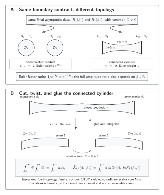
For the same two asymptotic JT boundary data, two disconnected disks contribute a product, whereas the connected genus-zero cylinder is obtained by gluing two trumpet exteriors along a closed geodesic of length $b$. Integrating one relative-twist period and the seam length produces $b\,db$. Since the cylinder has $\chi=0$, its Euler factor is suppressed by $e^{-2S_0}$ relative to two disks when $S_0\to\infty$ at fixed $\beta_i/C$; the full amplitude ratio also contains boundary-dependent coefficients. The connected term is present only when the topology, integration cycle, and fluctuation problem admit it. Its interpretation as an ensemble correlator requires the independently specified JT matrix-integral completion. Euclidean schematic, not to scale. Accessible figure data (JSON)

Case	Fixed boundary data	Topology	Integrated variables	Euler weight	Amplitude term	Admission condition	Licensed conclusion
Disconnected disks	$\beta_1,\beta_2$	$\mathcal D_1\sqcup\mathcal D_2$	One-boundary modes in each component	$\chi_{\rm total}=2$, $e^{2S_0}$	$e^{2S_0}\widehat Z_{0,1}(\beta_1)\widehat Z_{0,1}(\beta_2)$	Component-factorizing preparation and measure	Product contribution at genus zero.
Admitted double trumpet	$\beta_1,\beta_2$	Connected cylinder $\mathcal M_{0,2}$	$b\in(0,\infty)$ and one twist period $\theta\in[0,b)$	$\chi=0$, weight $1$	$\int_0^\infty b\,db\,Z_{\mathrm T}(\beta_1,b)Z_{\mathrm T}(\beta_2,b)$	Topology admitted and its fixed-topology integral defined	A connected Euclidean contribution in this prescription.
Connected topology excluded	$\beta_1,\beta_2$	Not in the sum	None	None	$0$	Topology policy omits $\mathcal M_{0,2}$	No cylinder term, even though the geometry can be described formally.
Zero cycle coefficient	$\beta_1,\beta_2$	Formal connected configuration	Formal moduli only	Not realized in the integral	$n_{\rm wh}=0$	Declared parent cycle has zero intersection	No contribution on that cycle.
Unresolved physical negative mode	$\beta_1,\beta_2$	Candidate connected sector	Mode and moduli treatment incomplete	Premature	Not a justified real-positive number	No descent prescription or stability control	Formal configuration only; contribution and dominance unresolved.

Scaling relative to two disks

For a connected orientable surface of genus $g$ with $n$ boundaries,

$$\chi=2-2g-n, \qquad Z_{g,n}=e^{S_0\chi}\widehat Z_{g,n}.$$

At genus zero, two disconnected disks have total Euler characteristic $2$, whereas the connected cylinder has $\chi=0$:

$$\begin{aligned} Z_{\mathrm{disc}}^{(0)} &=e^{2S_0}\widehat Z_{0,1}(\beta_1) \widehat Z_{0,1}(\beta_2),\\ Z_{\mathrm{conn}}^{(0)} &=\widehat Z_{0,2}(\beta_1,\beta_2). \end{aligned}$$

Therefore the topological suppression is $e^{-2S_0}$ as $S_0\to\infty$ with $\beta_i/C$ fixed. It is not the full ratio. With

$$\widehat Z_{0,1}(\beta) = \frac{C^{3/2}}{\sqrt{2\pi}\,\beta^{3/2}} \exp\!\left(\frac{2\pi^2C}{\beta}\right),$$

the complete leading ratio is

$$\frac{Z_{\mathrm{conn}}^{(0)}}{Z_{\mathrm{disc}}^{(0)}} =e^{-2S_0} \frac{(\beta_1\beta_2)^2}{C^3(\beta_1+\beta_2)} \exp\!\left[-2\pi^2C \left(\frac1{\beta_1}+\frac1{\beta_2}\right)\right].$$

At equal temperatures it becomes $e^{-2S_0}\frac{\beta^3}{2C^3}e^{-4\pi^2C/\beta}$. The $e^{-2S_0}$ hierarchy need not be uniform if $\beta_i/C$ themselves scale with $S_0$. This expression records the requested semiclassical scaling without confusing topological counting with temperature dependence. It also says nothing by itself about the convergence or uniqueness of the all-genus sum.

From a connected term to an interpretation

In the Saad–Shenker–Stanford matrix-integral completion, the perturbative connected correlator has the genus expansion

$$\big\langle Z(\beta_1)Z(\beta_2)\big\rangle_{c,\mathrm{pert}} \sim \sum_{g\geq0}e^{-2gS_0}\widehat Z_{g,2}(\beta_1,\beta_2),$$

whose $g=0$ term is the double trumpet. The brackets are not deduced from the cylinder: they are supplied by the independently constructed matrix integral, which is itself a nonunique nonperturbative completion of the asymptotic genus expansion Saad, Shenker, and Stanford 2019, abstract and §§1, 5.

For two decoupled copies of one specified Hamiltonian $H$, ordinary tensor-product reasoning instead gives

$$\operatorname{Tr}_{\mathcal H\otimes\mathcal H} e^{-\beta_1H\otimes1-\beta_2 1\otimes H} =Z_H(\beta_1)Z_H(\beta_2).$$

A semiclassical connected term then creates a factorization problem, not its own interpretation. Model studies at fixed couplings show how additional coupling-sensitive “half-wormhole” contributions can restore factorization while disappearing after averaging Saad, Shenker, Stanford, and Yao 2024, abstract and §§1–2. That is evidence for a mechanism in controlled models, not a theorem that every gravitational completion works this way. The detailed alternatives—fixed theory, ensemble, baby-universe state, or missing nonperturbative sector—belong to Factorization, Ensembles, and the Gravitational Path Integral and Baby Universes, Alpha Parameters, and Proposed Superselection Sectors.

Contour and stability stress tests

The strongest useful claim is the one that survives deliberate changes while all unrelated data remain fixed.

1. Topology test. Removing connected topology from the declared sum removes its contribution by definition. This compares different topology policies; it is not a dynamical proof that the geometry is absent.
2. Cycle test. Compute $n_s$ on the inherited parent cycle. If $n_s=0$, the formal saddle does not contribute. If a boundary source lies on a Stokes line, state the lateral prescription instead of averaging incompatible decompositions.
3. Spectrum test. Separate gauge, zero, positive, and physical negative modes. An unpaired negative mode blocks the naive real-positive determinant; only a specified thimble fixes its phase and meaning.
4. Complete-sum test. Add every contribution at the same approximation order. Cancellation can make the net cumulant vanish even when an individual connected term is nonzero.
5. UV test. Field-theoretic perturbative stability is weaker than stability against brane nucleation or other UV degrees of freedom.

The last distinction is visible in higher-dimensional examples. Under the Witten–Yau hypotheses, certain positive-Yamabe disconnected boundaries admit no smooth connected pure-Einstein filling; the exact domain and evasions are summarized on the boundary-condition page. Matter and sources can support Euclidean wormholes outside that obstruction. In ad hoc low-energy models, some branches can be perturbatively stable and dominate above a source threshold, while studied string compactifications retain brane-nucleation instabilities despite field-theoretic stability Marolf and Santos 2021, abstract and §§1, 7.

Even the field-theoretic negative-mode count depends on the boundary contract. A 2019 scalar-formulation analysis reported multiple negative modes for axion wormholes Hertog, Truijen, and Van Riet 2019, abstract, whereas a Lorentzian-path-integral analysis in the dual three-form description found perturbative stability Loges, Shiu, and Sudhir 2022, abstract. A later Euclidean reanalysis traced the discrepancy to the implementation of fixed axion charge, recovered agreement between the dual formulations, and found perturbative stability in its stated axion–saxion models Hertog et al. 2024, §3.3 and conclusion. The update does not prove UV stability; it shows why a claimed negative mode must name the fluctuating variables and what is fixed at infinity.

Contour relevance is equally model dependent. In a 2+1-dimensional axion model defined from a real Lorentzian contour, Held, Kaplan, Marolf, and Wang find source regions where the smooth Euclidean wormhole is subdominant to a UV-sensitive endpoint, regions where its ascent cycle does not intersect the integration contour, and a Stokes-line ambiguity for real positive axion data Held et al. 2026, abstract. The lesson is not that wormholes never contribute. It is that existence, cycle membership, dominance, and UV reliability are separate questions.

Evidence and claim ceiling

Result	Evidence class and domain	What survives	What does not follow
JT double-trumpet coefficient	Exact fixed-topology calculation in orientable pure JT with the stated normalization Saad, Shenker, and Stanford 2019, §3.4.1	The $b\,db$ integral, its finite coefficient, and $C$ cancellation.	One isolated full JT classical saddle.
JT matrix-integral dictionary	Perturbative genus expansion plus a specified, nonunique matrix completion Saad, Shenker, and Stanford 2019, §§1, 5	Connected JT amplitudes become connected matrix-ensemble correlators in that completion.	A universal ensemble interpretation for arbitrary gravity.
Higher-dimensional wormholes	Model- and source-dependent semiclassical examples Maldacena and Maoz 2004, §§1–2; Marolf and Santos 2021, §§1, 7	Existence, perturbative stability, or dominance in the explicitly tested regime.	UV stability or a complete exact amplitude.
Axion fluctuation spectrum	Boundary-condition-sensitive analyses with a documented correction Hertog, Truijen, and Van Riet 2019, abstract; Loges, Shiu, and Sudhir 2022, abstract; Hertog et al. 2024, §3.3	Fixing charge or flux consistently can change the physical negative-mode conclusion and reconcile dual formulations in the tested models.	Boundary-condition-independent stability or UV completion.
Fixed-coupling completion mechanism	Controlled toy and SYK-like models Saad, Shenker, Stanford, and Yao 2024, §§1–2	Additional saddles can restore fixed-coupling factorization in those models.	A universal gravitational cancellation theorem.
Constrained wormhole observables	Semiclassical constrained-instanton analysis Cotler and Jensen 2021, abstract and §§1–2	Smeared or transformed spectral observables may admit macroscopic saddle control.	UV control of the unsmeared full amplitude.
Real-contour axion test	Current model-specific preprint, submitted January 2026 Held et al. 2026, abstract	Intersection numbers, endpoints, and Stokes data can overturn a geometry-only inference.	The same contour answer for other matter or dimensions.
Reflection-positive fixed-$\alpha$ reconstruction	Current structural theorem that assumes a factorizing fixed-$\alpha$ partition function together with reflection positivity and completeness McNamara and Wang 2026, §1.1	Under those hypotheses, Hilbert-space and spatial-wormhole questions can be reconstructed from factorized boundary data.	Whether the multi-boundary Euclidean gravitational amplitude studied here factorizes, or how its contour should be evaluated.

The publication-safe conclusion is therefore conditional: a connected Euclidean sector contributes when the declared topology, boundary data, cycle coefficient, measure, and fluctuation problem admit it, and after same-order terms are summed it may produce a nonzero connected amplitude. An ensemble covariance, an exact fixed-theory answer, and Lorentzian traversability each require additional evidence.

Common pitfalls

A connected drawing is not a contribution. A geometry can solve local equations yet have zero intersection number, an excluded topology, an unresolved mode, or a larger competing contribution. Record the path-integral prescription before assigning it a weight.

A negative mode is not an automatic veto. It invalidates a naive positive Gaussian. The contour may supply a phase or an instability interpretation; without the contour, neither inclusion nor exclusion is justified.

The JT cylinder is not one isolated full saddle. Its finite answer is a gluing integral over $b$ and the twist quotient. Treating it as a single determinant around one classical JT solution erases the mechanism being calculated.

$e^{-2S_0}$ is not the whole ratio. It is only the Euler-weight suppression relative to two disks. The disk and cylinder coefficients bring additional $\beta_i/C$ dependence.

Connected does not mean ensemble averaged. Covariance notation requires a probability measure, while a fixed decoupled theory is expected to factorize. The mismatch is a problem to solve, not permission to rename the amplitude.

Exercises

1. Evaluate and check the double trumpet

Starting from the two trumpet factors, evaluate the $b$ integral and check convergence, exchange symmetry, $C$ independence, the equal-temperature value, and common rescaling of $\beta_1,\beta_2$.

Solution

Set

$$A=\frac{C(\beta_1+\beta_2)}{2\beta_1\beta_2}.$$

Then $\int_0^\infty b e^{-Ab^2}db=1/(2A)=\beta_1\beta_2/[C(\beta_1+\beta_2)]$. Multiplying by $C/(2\pi\sqrt{\beta_1\beta_2})$ gives

$$\widehat Z_{0,2} =\frac{\sqrt{\beta_1\beta_2}}{2\pi(\beta_1+\beta_2)}.$$

The integrand is $O(b)$ at the origin and Gaussian at infinity, so the integral converges. The answer is manifestly symmetric and contains no $C$. At $\beta_1=\beta_2=\beta$ it equals $1/(4\pi)$. Rescaling both thermal lengths by $\lambda>0$ multiplies numerator and denominator by $\lambda$, so the result is unchanged.

2. Separate Euler suppression from the full ratio

For a connected genus-$g$ surface with two boundaries, find its Euler weight relative to two disks. Explain why this is not the complete amplitude ratio.

Solution

The connected surface has $\chi=2-2g-2=-2g$ and weight $e^{-2gS_0}$. Two disks have total $\chi=2$ and weight $e^{2S_0}$. Their ratio is therefore

$$e^{-2(g+1)S_0}.$$

For the genus-zero cylinder this becomes $e^{-2S_0}$. The full ratio also divides the connected coefficient $\widehat Z_{g,2}$ by the product of disk coefficients, so it depends on $\beta_i/C$ and, beyond this benchmark, on sources, determinants, and moduli.

3. Recover a three-boundary cumulant

Assuming component-factorizing weights, express the fully connected three-boundary amplitude in terms of $Z_{123}$, the pair amplitudes, and the one-boundary amplitudes.

Solution

Subtract the three partitions with one connected pair and one singleton, then correct for subtracting the three-singleton partition three times rather than once:

$$Z_{123}^{c} =Z_{123}-Z_{12}Z_3-Z_{13}Z_2-Z_{23}Z_1 +2Z_1Z_2Z_3.$$

This Möbius inversion on set partitions isolates configurations whose connected component meets all three labeled boundaries. It fails to have this purely topological meaning if the disconnected measure or preparation does not factorize.

4. Fixed theory versus a two-member ensemble

An ensemble chooses theories $a$ and $b$ with probabilities $p$ and $1-p$. Derive the covariance of their two thermal partition functions and contrast it with two decoupled copies of one fixed Hamiltonian.

Solution

Writing $Z_r^{(i)}$ for boundary $i$ in realization $r$, direct expansion gives

$$\operatorname{Cov}(Z_1,Z_2) =p(1-p) \bigl(Z_a^{(1)}-Z_b^{(1)}\bigr) \bigl(Z_a^{(2)}-Z_b^{(2)}\bigr).$$

This can be nonzero because both observables share the same random realization. For two decoupled copies of one specified $H$, there is no probability measure to average over and the trace on $\mathcal H\otimes\mathcal H$ factorizes exactly into $Z_H(\beta_1)Z_H(\beta_2)$.

5. Apply the contour adversary

A regular connected solution exists for fixed sources. Classify the strongest surviving statement when (a) its topology is excluded, (b) its thimble intersection number is zero, (c) it has an unresolved physical negative mode, or (d) the sources are changed.

Solution

In (a), it is a formal solution of a topology not summed, so its amplitude contribution is zero by definition. In (b), it is an admitted formal saddle but contributes zero on the inherited cycle. In (c), it is a candidate contribution, but the naive real-positive Gaussian and any dominance claim are unjustified until a descent cycle fixes the phase or instability interpretation. In (d), one must solve the new boundary-value problem: neither existence nor coefficient carries over automatically. Only after topology, cycle, modes, measure, and the complete same-order sum are controlled may one claim a semiclassical contribution or dominance.

Continue to Semiclassical Gravitational Replicas for replicated boundary conditions, then to Replica Wormholes and Saddle Competition for entropy saddles. Baby-universe and exact factorization interpretations remain on their dedicated pages linked above.

The chapter overview contains the structure diagram and validity and failure diagram. They are embedded there once so that their shared chapter-level context is not repeated on every article.

For the chapter-wide comparison of assumptions, counterevidence, falsifiers, and claim ceilings, see the claim-domain table.

References

• Cotler, Jordan, and Kristan Jensen. “Wormholes and Black Hole Microstates in AdS/CFT.” Journal of High Energy Physics 2021, 9 (2021): 001. DOI; arXiv:2104.00601.
• Held, Jesse, Molly Kaplan, Donald Marolf, and Zhencheng Wang. “Axion Wormholes and the AdS/CFT Factorization Problem.” arXiv:2601.02507.
• Hertog, Thomas, Simon Maenaut, Bruno Missoni, Rob Tielemans, and Thomas Van Riet. “Stability of Axion-Saxion Wormholes.” Journal of High Energy Physics 2024, 11 (2024): 151. DOI; arXiv:2405.02072.
• Hertog, Thomas, Brecht Truijen, and Thomas Van Riet. “Euclidean Axion Wormholes Have Multiple Negative Modes.” Physical Review Letters 123 (2019): 081302. DOI; arXiv:1811.12690.
• Loges, Gregory J., Gary Shiu, and Nidhi Sudhir. “Complex Saddles and Euclidean Wormholes in the Lorentzian Path Integral.” Journal of High Energy Physics 2022, 8 (2022): 064. DOI; arXiv:2203.01956.
• Maldacena, Juan, and Liat Maoz. “Wormholes in AdS.” Journal of High Energy Physics 2004, 2 (2004): 053. DOI; arXiv:hep-th/0401024.
• Marolf, Donald, and Jorge E. Santos. “AdS Euclidean Wormholes.” Classical and Quantum Gravity 38 (2021): 224002. DOI; arXiv:2101.08875.
• McNamara, Jacob, and Zhencheng Wang. “Wormholes as Red Herrings: Reflection Positivity and the Reconstruction of Unitary Quantum Field Theories.” arXiv:2607.01322.
• Saad, Phil, Stephen H. Shenker, Douglas Stanford, and Shunyu Yao. “Wormholes without Averaging.” Journal of High Energy Physics 2024, 10 (2024): 076. DOI; arXiv:2103.16754.
• Saad, Phil, Stephen H. Shenker, and Douglas Stanford. “JT Gravity as a Matrix Integral.” arXiv:1903.11115.
• Witten, Edward, and Shing-Tung Yau. “Connectedness of the Boundary in the AdS/CFT Correspondence.” Advances in Theoretical and Mathematical Physics 3 (1999): 1635–1655. DOI; arXiv:hep-th/9910245.