Global, Poincaré, and AdS-Rindler Patches

Global, Poincaré, and AdS-Rindler coordinates describe overlapping regions of the same pure AdS geometry, but they organize different boundary domains and different time generators. Global coordinates cover the universal cover, the Poincaré chart ends on one Minkowski conformal patch, and an AdS-Rindler chart is adapted to the causal development of a boundary ball. A patch horizon is smooth in pure AdS; it limits the chart and the associated observable algebra, not the spacetime curvature.

Required background. Anti-de Sitter geometry and its conformal boundary supplies the embedding, compactified cylinder, and site-specific curvature signs. Helpful background. Causal, Killing, trapping, and apparent horizons distinguishes a coordinate Killing horizon from invariant singular or trapped structure.

Three charts, three boundary domains

Throughout, the Lorentzian signature is $(+,-,\ldots,-)$, the AdS radius is $L$, and $d\geq2$. The $d=1$ exception is stated below rather than hidden inside formulas that use a boundary sphere or ball. The essential comparison is:

Coordinate coverage, time generators, and chart horizons in pure AdS

Chart	Boundary representative and domain	Time generator	Interior edge of the chart
global	ℝτ × Sd−1, the full boundary cylinder	∂τ, conjugate to cylinder energy	none on the universal cover
Poincaré	ℝ1,d−1, one conformal diamond of the cylinder	∂t, conjugate to Minkowski energy	the null Poincaré horizon
AdS-Rindler	ℝη × Hd−1, conformal to a ball’s causal diamond	∂η, the hyperbolic-time generator	a bifurcate Killing horizon

The entries in the last two rows are coordinate boundaries, not curvature singularities. State preparation and boundary conditions still have to be supplied before a mode basis becomes a quantum vacuum or a thermal ensemble.

The coverage map makes both restrictions visible. Read its upper row from left to right: a cylinder diamond becomes the full Minkowski representative, then a ball diamond becomes the full hyperbolic cylinder. Its lower row records the matching bulk condition, time generator, and smooth inner edge. The signed angle $\vartheta$ in the figure runs along a boundary great circle; it is not the bulk radial coordinate $\chi$ used later.

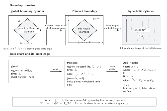
For pure AdS$_{d+1}$ with $d\geq2$, the principal Poincaré diamond on the boundary cylinder maps to all finite points of one Minkowski representative, while a centered ball’s causal diamond maps to $\mathbb R_\eta\times H^{d-1}$. The displayed time generators are $\partial_\tau$, $\partial_t$, and $\partial_\eta$. In the bulk the selected lift has $X^+>0$, while the AdS-Rindler chart has $\varrho>1$ and covers the causal wedge $X_d>\lvert X_0\rvert$, $X_{-1}>0$. Its invariant edges are $X^+=0$ for the Poincaré chart and $X_d=\pm X_0$ with $X_d\geq0$ for the AdS-Rindler chart; $\varrho=1$ at finite $\eta$ is only the latter pair’s bifurcation surface. These are smooth null horizons of the same spacetime with $\mathcal R=d(d+1)/L^2$ in the site convention. The figure suppresses transverse directions and is schematic, not to scale.

From the global hyperboloid to a Poincaré patch

Global coordinates give

$$\mathrm ds^2=L^2\left( \cosh^2\rho\,\mathrm d\tau^2 -\mathrm d\rho^2 -\sinh^2\rho\,\mathrm d\Omega_{d-1}^2 \right).$$

They cover the entire universal cover, with conformal boundary $\mathbb R_\tau\times S^{d-1}$. To isolate a Poincaré patch, define the null ambient combination

$$X^+\equiv X_{-1}+X_d$$

and restrict to $X^+>0$. This notation avoids confusing the ambient null component with the projective boundary vector used on the prerequisite page. With $x^\mu=(t,\mathbf x)$ and $x^2=t^2-\lvert\mathbf x\rvert^2$, set

$$z=\frac{L^2}{X^+}, \qquad x^\mu=\frac{L X^\mu}{X^+}, \qquad z>0,$$

where $X^\mu=(X_0,X_1,\ldots,X_{d-1})$. The inverse map is

$$\begin{aligned} X_{-1}&=\frac{L^2+z^2-x^2}{2z}, &X_d&=\frac{L^2-z^2+x^2}{2z},\\ X^\mu&=\frac{Lx^\mu}{z}. \end{aligned}$$

Substitution into the ambient metric gives

$$\mathrm ds^2=\frac{L^2}{z^2} \left(\mathrm dt^2-\mathrm d\mathbf x^2-\mathrm dz^2\right).$$

On the universal cover, the embedding coordinates repeat under $\tau\mapsto\tau+2\pi$, so $X^+>0$ has infinitely many connected lifts that the tuple $(z,x^\mu)$ does not distinguish. Here and below, “the Poincaré patch” means the connected lift containing the $\tau=0$ slice. The hypersurface $z=0$ is its Minkowski representative of the conformal boundary.

The bulk chart horizon is the invariant null surface $X^+=0$. Reaching a finite point of it requires a correlated limit: as $z\to\infty$, both $x^\mu/z$ and $(x^2-z^2)/z$ must approach finite values. At fixed $(t,\mathbf x)$, by contrast, $z\to\infty$ approaches the compactified spatial-infinity corner of the Minkowski representative. Thus “$z=\infty$” alone does not identify a unique horizon point. Every curvature scalar remains at its pure-AdS value across the extended surface Aharony et al. 2000, §2.2.1, eqs. (2.26)–(2.28).

The boundary coverage can be seen without guessing. Choose a polar angle $\theta$ on the global $S^{d-1}$ so that $n_d=\cos\theta$. At the boundary,

$$\frac{t}{L}=\frac{\sin\tau}{\cos\tau+\cos\theta}, \qquad \frac{r_{\partial}}{L}=\frac{\sin\theta}{\cos\tau+\cos\theta},$$

with $r_{\partial}\equiv\lvert\mathbf x\rvert$ and $\cos\tau+\cos\theta>0$. This is one diamond on the global cylinder. The open future and past edges map to $\mathscr I^+$ and $\mathscr I^-$; its future and past tips map to $i^+$ and $i^-$, and the remaining corner maps to spatial infinity $i^0$. None is an additional finite point of $\mathbb R^{1,d-1}$.

AdS$_2$ exception. When $d=1$, the global boundary has two timelike components rather than a spatial sphere carrying a diamond, and its one-dimensional boundary metric has no null edges. The selected Poincaré chart reaches one component with $t/L=\tan(\tau/2)$ for $-\pi<\tau<\pi$. The spherical-ball modular construction used below also degenerates because $H^0$ is a point, so this page’s remaining ball and hyperbolic formulas are stated only for $d\geq2$.

An explicit global mode in Poincaré coordinates

For a free Klein–Gordon field obeying $(\Box+m^2)\phi=0$, let

$$m^2L^2=\Delta(\Delta-d), \qquad \Delta=\Delta_+=\frac d2+\sqrt{\frac{d^2}{4}+m^2L^2}.$$

Assume the Breitenlohner–Freedman stability bound $m^2L^2\geq-d^2/4$, so $\Delta_+$ is real Aharony et al. 2000, §2.2.2, eq. (2.42). With standard quantization, regular reflecting boundary conditions, and $d\geq2$, the stable global normal modes have dimensionless frequencies Aharony et al. 2000, §2.2.2, eq. (2.41)

$$\omega_{n\ell}=\Delta+2n+\ell, \qquad n,\ell=0,1,2,\ldots.$$

The lowest spherically symmetric mode may be written, up to normalization, as

$$\phi_0(\tau,\rho)=e^{-i\Delta\tau}(\cosh\rho)^{-\Delta}.$$

Because

$$\cosh\rho\,e^{i\tau}=\frac{X_{-1}+iX_0}{L},$$

the coordinate map gives the exact expression on the Poincaré overlap,

$$\phi_0(z,t,\mathbf x) =\left[ \frac{2Lz} {L^2+z^2-x^2+2iLt} \right]^\Delta.$$

Near $z=0$, this standard-quantization solution has the expansion

$$\phi_0(z,t,\mathbf x) =z^\Delta\beta(t,\mathbf x)\left[1+\mathcal O(z^2)\right],$$

where the normalizable coefficient is

$$\beta(t,\mathbf x) =\left[ \frac{2L} {L^2-t^2+\lvert\mathbf x\rvert^2+2iLt} \right]^\Delta.$$

For noninteger $\Delta$, these equalities are defined on the chosen lift with the branch inherited continuously from $\arg(X_{-1}+iX_0)=\tau$ on $-\pi<\tau<\pi$. Moving to the lift shifted by $2\pi k$ multiplies the global mode by $e^{-2\pi i k\Delta}$; the bare coordinates $(z,x^\mu)$ do not remember that phase. The same inherited branch is used in $\beta(t,\mathbf x)$, so no independent Poincaré prescription has been introduced.

This calculation does more than relabel the metric. A single global-energy eigenmode becomes a wavepacket—a continuous superposition of Poincaré-energy eigenmodes—because $\partial_\tau$ and $\partial_t$ are different $SO(2,d)$ generators. The classical field agrees point by point on the overlap, while its spectral decomposition and accessible boundary support change.

Different generators do not automatically imply different invariant vacua. For this free field on fixed AdS, the $SO(2,d)$-invariant Fock vacuum is one state expressed in different regional mode bases. Holographically, it is the bulk representative of the cylinder CFT vacuum, whose conformal image is the ordinary Minkowski vacuum. What changes here is the mode basis and domain. A vacuum defined only by an unrelated positive-frequency prescription would require a separate state comparison.

AdS-Rindler coordinates and a boundary ball

The AdS-Rindler chart can be derived directly from the same embedding. Let $\hat n_a$ be a unit vector on $S^{d-2}$ and set

$$\begin{aligned} X_{-1}&=L\varrho\cosh u, &X_a&=L\varrho\sinh u\,\hat n_a, &&a=1,\ldots,d-1,\\ X_0&=L\sqrt{\varrho^2-1}\sinh\eta, &X_d&=L\sqrt{\varrho^2-1}\cosh\eta. \end{aligned}$$

For $\varrho>1$ and $u\geq0$, these coordinates cover the connected wedge

$$X_d>\lvert X_0\rvert, \qquad X_{-1}>0.$$

On the universal cover these ambient inequalities recur on different $2\pi$ global-time lifts. Here “the AdS-Rindler wedge” means the component containing the $\tau=0$ slice, matching the Poincaré lift fixed above.

Substitution into the ambient metric gives

$$\mathrm ds^2=L^2\left[ (\varrho^2-1)\,\mathrm d\eta^2 -\frac{\mathrm d\varrho^2}{\varrho^2-1} -\varrho^2\,\mathrm dH_{d-1}^2 \right], \qquad \varrho>1.$$

The boost in the $(X_0,X_d)$ plane is the chart’s time translation:

$$k_\eta=\partial_\eta =X_d\partial_{X_0}+X_0\partial_{X_d}, \qquad k_\eta^2=X_d^2-X_0^2=L^2(\varrho^2-1).$$

It is timelike inside the wedge and null on its boundary. The future and past branches are

$$\mathcal H^+: X_d=X_0\geq0,\quad X_{-1}>0, \qquad \mathcal H^-: X_d=-X_0\geq0,\quad X_{-1}>0.$$

The coordinate value $\varrho=1$ at finite $\eta$ gives only their bifurcation surface $X_0=X_d=0$, which is isometric to $H^{d-1}$. Points away from that surface are reached by sending $\varrho\to1$ and $\eta\to\pm\infty$ together while keeping the appropriate product $\sqrt{\varrho^2-1}\,e^{\lvert\eta\rvert}$ finite. This distinction prevents the collapsed static coordinate from being mistaken for the whole horizon.

Regularity is also explicit. Writing $\varrho=\cosh\chi$ gives

$$\mathrm ds^2=L^2\left[ \sinh^2\chi\,\mathrm d\eta^2 -\mathrm d\chi^2 -\cosh^2\chi\,\mathrm dH_{d-1}^2 \right].$$

Near $\chi=0$, the $(\eta,\chi)$ part is ordinary Rindler space, $L^2(\chi^2\mathrm d\eta^2-\mathrm d\chi^2)$. Define

$$T=\chi\sinh\eta, \qquad Y=\chi\cosh\eta.$$

Then $\chi^2\mathrm d\eta^2-\mathrm d\chi^2=\mathrm dT^2-\mathrm dY^2$: the apparently degenerate static coordinates are simply one Minkowski wedge, and $T=\pm Y$ gives its smooth null extension. In addition,

$$R_{MNPQ}R^{MNPQ}=\frac{2d(d+1)}{L^4}$$

remains finite and constant. The horizon is therefore a coordinate Killing horizon, not a curvature singularity. With the dimensionless generator $\partial_\eta$, its surface gravity is $1$; normalizing the boundary physical time as $\tau_H=R\eta$ gives surface gravity $1/R$.

Its conformal boundary is $\mathbb R_\eta\times H^{d-1}$. To connect the bulk wedge to a boundary ball, write

$$\mathrm dH_{d-1}^2 =\mathrm du^2+\sinh^2u\,\mathrm d\Omega_{d-2}^2$$

and define

$$D_\varrho =\varrho\cosh u +\sqrt{\varrho^2-1}\cosh\eta.$$

The embedding-to-Poincaré map then becomes

$$\frac zR=\frac1{D_\varrho}, \qquad \frac tR=\frac{\sqrt{\varrho^2-1}\sinh\eta}{D_\varrho}, \qquad \frac rR=\frac{\varrho\sinh u}{D_\varrho}.$$

The direct embedding has $R=L$; an arbitrary ball radius follows from the Poincaré dilation $(t,\mathbf x,z)\mapsto(R/L)(t,\mathbf x,z)$. Taking $\varrho\to\infty$ gives the boundary map

$$\frac{t}{R}=\frac{\sinh\eta}{\cosh u+\cosh\eta}, \qquad \frac{r}{R} =\frac{\sinh u}{\cosh u+\cosh\eta}.$$

For the radial null coordinates $x^\pm=t\pm r$,

$$\frac{x^\pm}{R} =\tanh\!\left(\frac{\eta\pm u}{2}\right).$$

Both ratios lie strictly between $-1$ and $1$, so the image is exactly the ball’s causal diamond $\lvert t\rvert+r<R$. The metric relation is

$$\mathrm ds_{\mathrm M}^2 =\frac{R^2}{(\cosh u+\cosh\eta)^2} \left(\mathrm d\eta^2-\mathrm dH_{d-1}^2\right).$$

On the diamond, the same flow is generated by the conformal Killing field

$$\xi_\eta=\partial_\eta =\frac{R^2-t^2-r^2}{2R}\,\partial_t -\frac{t}{R}x^i\partial_i,$$

whose norm factorizes as

$$\xi_\eta^2 =\frac{[R^2-(t+r)^2][R^2-(t-r)^2]}{4R^2}.$$

It is timelike precisely inside the diamond and null on its boundary. Thus AdS-Rindler time is adapted to a ball-preserving conformal flow, not to global or Minkowski time translation Casini, Huerta, and Myers 2011, §2.2, eqs. (27)–(33).

Now specify the state. With a UV regulator that supplies a type-I factorization, the CFT vacuum reduced to the ball has modular Hamiltonian

$$K_B=-\log\rho_B =2\pi\!\int_{\lvert\mathbf x\rvert<R}\!\mathrm d^{d-1}x\, \frac{R^2-\lvert\mathbf x\rvert^2}{2R} T_{00}(0,\mathbf x)+c_B,$$

where $c_B$ fixes $\operatorname{Tr}\rho_B=1$ Casini, Huerta, and Myers 2011, §2.1, eq. (22). Let $U$ denote the conformal identification of the ball diamond with the hyperbolic cylinder, and let $H_\eta$ generate translations of the dimensionless coordinate $\eta$. Then

$$U\rho_B U^{-1}=\rho_H=Z^{-1}e^{-2\pi H_\eta}, \qquad UK_BU^{-1}=2\pi H_\eta+\log Z,$$

with $Z=\operatorname{Tr}e^{-2\pi H_\eta}$ in that regulated description. Since $H_\eta=R H_{\mathrm{hyp}}$ for physical hyperbolic time $\tau_H=R\eta$, the inverse temperature is $\beta_H=2\pi R$ and

$$T_H=\frac1{2\pi R}.$$

The sign of geometric modular flow must be declared. With the site convention

$$\sigma_s(A)=\Delta_B^{is}A\Delta_B^{-is},$$

and $\alpha_\eta(A)=e^{iH_\eta\eta}Ae^{-iH_\eta\eta}$, one has $\sigma_s=\alpha_{-2\pi s}$. With the site’s positive-upper-strip convention, the vacuum is Kubo–Martin–Schwinger (KMS) at inverse temperature $\beta_\eta=2\pi$ for the geometric flow $\alpha_\eta$. Equivalently, it is unit-temperature KMS for the inverse modular group $\sigma_{-s}=\alpha_{+2\pi s}$.

In continuum QFT, the local algebra is generally type III, so a canonical Hilbert-space tensor factor for the ball, a trace-class $\rho_B$, and $Z$ are regulator-dependent shorthand Witten 2018, §§2.5 and 6.4–6.5. The intrinsic statement is that the vacuum restricted to the ball algebra has the modular/KMS flow above Witten 2018, §§3 and 4.2. The site’s rigorous modular-dynamics treatment fixes the represented algebra and sign convention. A faithful normal state determines a modular group; with the convention declared here, its positive-strip KMS dynamics is the inverse modular group. The special claim for the vacuum is thermality under the fixed geometric $\eta$-flow generated by $H_\eta$. A generic excited state need not have that geometric KMS property merely because the chart has a Killing horizon.

The wedge is the causal wedge of the boundary diamond in pure AdS. Its complement contains bulk points that cannot both send a signal to and receive a signal from that diamond. Hamilton et al. give an explicit free-scalar reconstruction in AdS$_3$ Rindler coordinates and discuss its implications Hamilton et al. 2006, §§4–5. Higher-dimensional or interacting reconstruction requires separately stated field, boundary, state, and code-sector hypotheses.

Coverage, completeness, and regularity checks

Tests that separate coordinate, mode, state, and reconstruction claims

Proposed conclusion	Check that must be performed	Strongest conclusion if the check passes
“the chart ends at a singularity”	evaluate a curvature invariant and extend the embedding coordinates	only the coordinate chart ends at a smooth null surface
“these modes are complete”	name the region, function space, inner product, and boundary or horizon condition	completeness for that declared regional problem
“the wedge algebra determines the global state”	compare correlations with the complementary diamond and specify any reconstruction theorem	generally only the restricted state is fixed
“the horizon makes the state thermal”	verify the KMS condition for the chosen state, algebra, and Killing flow	thermality relative to that generator and algebra
“a patch source fixes a global solution”	supply regularity, analyticity, or data on the omitted boundary region	a continuation under those additional hypotheses

These tests separate three questions that are often conflated: whether coordinates are regular, whether a mode expansion is complete for a regional boundary problem, and whether a chosen quantum state is thermal with respect to the chart’s Hamiltonian.

Common pitfalls

Calling every $z\to\infty$ limit the Poincaré horizon—or a singularity. The invariant bulk edge is $X^+=0$, and finite horizon points require the correlated scaling stated above. Fixed $(t,\mathbf x)$ instead approaches the compactified $i^0$ corner. Neither limit creates a curvature singularity in pure AdS.

Promoting a regional mode basis to global completeness. The Poincaré and AdS-Rindler bases solve problems on smaller domains. Extending them globally requires the missing boundary, horizon, and state data.

Inferring thermality from geometry alone. The vacuum restricted to a ball has the special KMS property above for the geometric $\eta$-flow. The same wedge chart can be used for excited states that are not KMS with respect to that fixed flow. A faithful normal state still determines its own modular group; under the site convention the corresponding positive-strip KMS dynamics is the inverse modular group.

Exercises

Locate the Minkowski patch on the cylinder

Use the boundary map to show that the denominator $\cos\tau+\cos\theta$ is positive precisely inside one conformal diamond, and that its zero set is null in the cylinder metric.

Solution: cylinder diamond

On the principal interval $-\pi<\tau<\pi$ with $0\leq\theta\leq\pi$,

$$\cos\tau+\cos\theta =2\cos\frac{\tau+\theta}{2} \cos\frac{\tau-\theta}{2}.$$

Both factors are positive when $\lvert\tau\rvert+\theta<\pi$. The equations $\tau+\theta=\pi$ and $\tau-\theta=-\pi$ give the future and past branches of the principal diamond; their $2\pi$ translates bound the other lifts. Radial curves obey $\mathrm ds_{\partial}^2=\mathrm d\tau^2-\mathrm d\theta^2$, so $\mathrm d\tau=\pm\mathrm d\theta$ on these edges: they are null. Their open segments map to $\mathscr I^\pm$, while the vertices map to $i^+$, $i^-$, and $i^0$.

Check the transformed ground mode

On the connected lift containing $\tau=0$, substitute the inverse Poincaré map into $(X_{-1}+iX_0)^{-\Delta}$ and recover the displayed $\phi_0(z,t,\mathbf x)$. Explain why it is not a single eigenmode of $i\partial_t$, and state what changes on the lift shifted by $2\pi k$.

Solution: transformed global mode

The inverse map gives

$$X_{-1}+iX_0 =\frac{L^2+z^2-x^2+2iLt}{2z}.$$

Since $\phi_0=L^\Delta(X_{-1}+iX_0)^{-\Delta}$ on the branch continuously inherited from $-\pi<\tau<\pi$, the Poincaré expression follows immediately. Acting with $i\partial_t$ differentiates a nonexponential rational power, so the result is not a constant times $\phi_0$. Its Fourier representation is therefore a superposition of Poincaré energies. On the lift $\tau\mapsto\tau+2\pi k$, the global factor $e^{-i\Delta\tau}$ contributes the phase $e^{-2\pi i k\Delta}$, which is not encoded by $(z,x^\mu)$ alone.

Derive the AdS-Rindler wedge and its boundary diamond

Starting from the AdS-Rindler embedding, verify the hyperbolic metric and $k_\eta^2=L^2(\varrho^2-1)$. Then take the boundary limit of the bulk Poincaré map, derive $x^\pm/R=\tanh[(\eta\pm u)/2]$, and recover both the Weyl factor and the domain $\lvert t\rvert+r<R$. Finally, explain why $\varrho=1$ is not a curvature singularity.

Solution: ball diamond and smooth horizon

Differentiating the four embedding expressions and using $\hat n_a\hat n_a=1$ and $\hat n_a\mathrm d\hat n_a=0$ gives

$$\mathrm ds^2=L^2\left[ (\varrho^2-1)\mathrm d\eta^2 -\frac{\mathrm d\varrho^2}{\varrho^2-1} -\varrho^2\mathrm dH_{d-1}^2 \right].$$

The ambient boost generator is $k_\eta=X_d\partial_{X_0}+X_0\partial_{X_d}$, so its norm is $X_d^2-X_0^2=L^2(\varrho^2-1)$. At the boundary, put $D=\cosh u+\cosh\eta$. The identities

$$D=2\cosh\frac{\eta+u}{2}\cosh\frac{\eta-u}{2}, \qquad \sinh\eta\pm\sinh u =2\sinh\frac{\eta\pm u}{2}\cosh\frac{\eta\mp u}{2}$$

give

$$\frac{x^\pm}{R} =\frac{\sinh\eta\pm\sinh u}{D} =\tanh\frac{\eta\pm u}{2}.$$

Hence $-R<x^\pm<R$, which is equivalent to $\lvert t\rvert+r<R$. Direct differentiation yields

$$\mathrm ds_{\mathrm M}^2 =\frac{R^2}{D^2} \left(\mathrm d\eta^2-\mathrm dH_{d-1}^2\right).$$

Finally, $\varrho=\cosh\chi$ gives $\chi^2\mathrm d\eta^2-\mathrm d\chi^2$ near the horizon. With $T=\chi\sinh\eta$ and $Y=\chi\cosh\eta$, this is $\mathrm dT^2-\mathrm dY^2$, so the chart extends smoothly across $T=\pm Y$. The constant invariant $R_{MNPQ}R^{MNPQ}=2d(d+1)/L^4$ independently rules out a curvature singularity.

Separate a chart horizon from a thermal state

Keep the same AdS-Rindler wedge but replace the vacuum by a generic excited CFT state. Which statements on this page remain geometric, and what must be checked before calling the restricted state thermal?

Solution: geometry versus state

The embedding domain, metric, conformal boundary, Killing field, bifurcate horizon, ball-preserving conformal flow, and constant curvature are unchanged. Thermality with respect to the fixed geometric $\eta$-flow is not. One must specify the regional algebra and state and verify the KMS strip condition for the $H_\eta$ evolution. A regulated density matrix may then be compared with $e^{-2\pi H_\eta}$; in continuum QFT, with the site convention above, the intrinsic test compares the state’s inverse modular group with the positive geometric flow rather than assuming a trace-class reduced density matrix.

Timelike-Boundary Causality and Boundary-Value Problems now fixes the boundary data needed for evolution. Later, bulk reconstruction and locality asks what boundary region can reconstruct which bulk observables.

The chapter overview contains the structure diagram and validity and failure diagram. They are embedded there once so that their shared chapter-level context is not repeated on every article.

For the chapter-wide comparison of assumptions, counterevidence, falsifiers, and claim ceilings, see the claim-domain table.

References

• Aharony, Ofer, Steven S. Gubser, Juan Maldacena, Hirosi Ooguri, and Yaron Oz. “Large N Field Theories, String Theory and Gravity.” Physics Reports 323 (2000): 183–386. arXiv. DOI.
• Casini, Horacio, Marina Huerta, and Robert C. Myers. “Towards a Derivation of Holographic Entanglement Entropy.” Journal of High Energy Physics 2011, 036 (2011). arXiv. DOI.
• Hamilton, Alex, Daniel Kabat, Gilad Lifschytz, and David A. Lowe. “Holographic Representation of Local Bulk Operators.” Physical Review D 74 (2006): 066009. arXiv. DOI.
• Witten, Edward. “Notes on Some Entanglement Properties of Quantum Field Theory.” Reviews of Modern Physics 90 (2018): 045003. arXiv. DOI.