Absorption, Emission, and Dynamical Tests

Counting states tests a density of levels. Absorption and emission test something stricter: normalized matrix elements as functions of frequency, polarization, state, and resolution. This page works through one classic success—the neutral, minimally coupled $s$-wave of the near-extremal D1–D5–P black hole—and keeps its claim deliberately narrow. In the dilute-gas, low-energy regime, a bulk flux calculation and a thermal D1–D5 CFT response give the same five-dimensional cross section and emission rate. The result does not describe every scalar, every frequency, or the line-by-line response of an individual finite-volume microstate.

Required background. D-Brane Bound States and the Strominger–Vafa Count fixes the brane system and the weak/strong-coupling comparison. D1–D5 CFT and AdS₃ Microstate Data supplies the Ramond-sector dictionary, the long-string description, and the distinction between protected and unprotected CFT data.

Helpful background. Boulware, Hartle–Hawking, and Unruh States separates a state label from an observed flux. Ray Tracing and the Hawking Bogoliubov Map owns the origin of Hawking occupation numbers. Greybody Scattering and Flux Accounting develops the general radial-scattering normalization used here.

On this page. Follow the model and regime, bulk flux calculation, normalized CFT response, emission relation, area and numerical checks, finite-volume interpretation, failure tests, or solved exercises.

The D1–D5 response test and its regime

Take type-IIB string theory on $T^4\times S^1$. The five-dimensional black hole carries D1, D5, and momentum charges. In the dilute-gas parametrization, $r_1$ and $r_5$ are the D1 and D5 charge radii, $r_0$ measures nonextremality, and the momentum charge is written

$$r_n=r_0\sinh\delta_p,$$

where $\delta_p$ is a boost parameter. The effective left- and right-moving temperatures are

$$T_L=\frac{r_0e^{\delta_p}}{2\pi r_1r_5}, \qquad T_R=\frac{r_0e^{-\delta_p}}{2\pi r_1r_5},$$

and therefore

$$T_H=\frac{r_0}{2\pi r_1r_5\cosh\delta_p}, \qquad \frac{2}{T_H}=\frac{1}{T_L}+\frac{1}{T_R}.$$

The worked channel is one neutral, massless minimal-scalar polarization arising, for example, from a traceless off-diagonal fluctuation of the $T^4$ metric. Write its canonically normalized five-dimensional fluctuation as $\delta\varphi_{\rm can}$; its dimensionless boundary source will be $\varphi_{\partial}=\kappa_5\delta\varphi_{{\rm can},\partial}$. It has zero Kaluza–Klein momentum along $S^1$ and angular momentum $\ell=0$ on the transverse $S^3$. These labels matter: changing them changes the radial equation, the CFT operator, or both.

The calculation uses the simultaneous hierarchy

$$r_0,r_n\ll r_1,r_5, \qquad \omega r_1\ll1, \qquad \omega r_5\ll1,$$

with $r_1/r_5=O(1)$ in the standard matched-asymptotic treatment. Supergravity additionally requires charge radii large compared with the string length and small loop and curvature corrections. The ratio $\omega/T_L$ or $\omega/T_R$ need not be small; retaining those ratios is exactly what preserves the nontrivial frequency dependence Maldacena and Strominger 1997, §§2–4, especially eqs. (2.7), (2.9), and (4.3).

Three quantities must not be conflated:

• $\mathcal P_0$ is the dimensionless $s$-wave absorption probability, obtained from a ratio of conserved radial fluxes.
• $\sigma_{\rm abs}$ is the plane-wave absorption cross section. In four noncompact spatial dimensions it has dimensions $L^3$.
• $d\Gamma_{\rm em}$ is an emission rate. It includes the cross section, a Hawking occupation factor, and final-state phase space.

The literature sometimes calls either $\mathcal P_0$ or $\sigma_{\rm abs}$ a “greybody factor.” The equations below keep the two normalizations explicit.

Bulk route: flux through the radial barrier

Write the selected canonical mode as $\delta\varphi_{\rm can}=e^{-i\omega t}R_\omega(r)$ and define

$$h(r)=1-\frac{r_0^2}{r^2}, \qquad f(r)= \left(1+\frac{r_n^2}{r^2}\right) \left(1+\frac{r_1^2}{r^2}\right) \left(1+\frac{r_5^2}{r^2}\right).$$

For the neutral minimal scalar, the five-dimensional Einstein-frame Klein–Gordon equation reduces to

$$\left[ \frac{h}{r^3}\frac{d}{dr} \left(hr^3\frac{d}{dr}\right) +\omega^2 f \right]R_\omega=0.$$

Its conserved radial flux is

$$\mathcal F_r= \frac{1}{2i} \left( R_\omega^*hr^3\frac{dR_\omega}{dr} -R_\omega hr^3\frac{dR_\omega^*}{dr} \right).$$

Impose a purely ingoing solution at the future horizon and decompose the large-$r$ solution into incident and reflected waves. Then

$$\mathcal P_0 =\frac{\lvert\mathcal F_{\rm hor}\rvert} {\lvert\mathcal F_{\rm in}\rvert}.$$

This is not yet the plane-wave cross section. The $s$-wave projection of a plane wave in four spatial dimensions supplies

$$\boxed{ \sigma_{\rm abs}(\omega)=\frac{4\pi}{\omega^3}\,\mathcal P_0(\omega) }.$$

The factor $\omega^{-3}$ is why a finite low-frequency cross section can coexist with $\mathcal P_0\to0$.

Near and far solutions share an overlap

For $r_1/r_5=O(1)$, choose a matching radius satisfying

$$\max\!\left(r_0,r_n,\omega r_1r_5\right) \ll r_m\ll \min\!\left(r_1,r_5,\omega^{-1}\right).$$

Thus both $\omega r_m\ll1$ and $\omega r_1r_5/r_m\ll1$ hold where the near and far expansions are compared. In the far region, $\rho=\omega r$ gives

$$R_{\rm far}(r)= \sqrt{\frac{\pi\omega}{2}}\frac{1}{r} \left[\alpha J_1(\omega r)+\beta N_1(\omega r)\right].$$

In the near region, $v=r_0^2/r^2$ reduces the radial equation to a hypergeometric equation. Its two useful parameters are

$$a=\frac{\omega}{4\pi T_R}, \qquad b=\frac{\omega}{4\pi T_L}.$$

Let $z=1-v=h(r)$. The solution normalized to be purely ingoing at the future horizon is

$$R_{\rm near}(z)= \mathcal A_h z^{-i(a+b)/2}, {}_2F_1(-ia,-ib;1-ia-ib;z).$$

In the overlap region $v\to0$, this becomes $R_{\rm near}=\mathcal A_hE+O(v\log v)$, with connection coefficient

$$E= \frac{\Gamma(1-ia-ib)} {\Gamma(1-ia)\Gamma(1-ib)}.$$

Matching both the field and its derivative gives

$$\sqrt{\frac{\pi}{2}}\omega^{3/2}\frac{\alpha}{2} =\mathcal A_hE, \qquad \frac{\beta}{\alpha}\ll1.$$

The incident and horizon flux magnitudes are therefore

$$\lvert\mathcal F_{\rm in}\rvert =\omega\left\lvert\frac{\alpha}{2}\right\rvert^2, \qquad \lvert\mathcal F_{\rm hor}\rvert =r_0^2(a+b)\lvert\mathcal A_h\rvert^2,$$

so the matching spine closes before any thermal rewriting:

$$\mathcal P_0 =\frac{\pi}{2}r_0^2(a+b)\omega^2\lvert E\rvert^{-2}.$$

The identity

$$\lvert\Gamma(1-ix)\rvert^2 =\frac{\pi x}{\sinh\pi x}$$

then converts $\lvert E\rvert^{-2}$ into thermal factors. After the plane-wave normalization above, the result is

$$\boxed{ \sigma_{\rm abs}(\omega) =\pi^3r_1^2r_5^2\omega\, \frac{e^{\omega/T_H}-1} {\left(e^{\omega/(2T_L)}-1\right) \left(e^{\omega/(2T_R)}-1\right)} }.$$

Equivalently, the absorption probability is

$$\mathcal P_0(\omega) =\frac{\pi^2}{4}r_1^2r_5^2\omega^4 \frac{e^{\omega/T_H}-1} {\left(e^{\omega/(2T_L)}-1\right) \left(e^{\omega/(2T_R)}-1\right)}.$$

This is the bulk calculation of Maldacena and Strominger 1997, §4, eqs. (4.1)–(4.35). The matching calculation controls the displayed leading term; it does not supply a rigorous error bar at a sharp value of $\omega r_{1,5}$.

CFT route: a thermal operator absorbs one quantum

The same bulk scalar couples to a D1–D5 CFT operator $\mathcal O$ of weights $(h_L,h_R)=(1,1)$:

$$S_{\rm int}=\mu\int dt\,dy\, \varphi_{\partial}(t,y)\mathcal O(t,y).$$

If the zero-temperature two-point function is normalized by

$$\langle\mathcal O(x^+,x^-)\mathcal O(0)\rangle =\frac{C_{\mathcal O}} {(x^+-i\epsilon)^2(x^--i\epsilon)^2}, \qquad x^\pm=t\pm y,$$

then the rate depends on the invariant product $\mu^2C_{\mathcal O}$. A proportional correlator fixes the frequency and temperature dependence but not the absolute cross section. With the notation fixed above,

$$S_{\rm int} =\int d^2x\,\varphi_{\partial}\mathcal O =\kappa_5\int d^2x\,\delta\varphi_{{\rm can},\partial}\mathcal O.$$

Thus $\mu=1$ in the dimensionless-source convention, while the canonical-field convention displays $\kappa_5$ David, Mandal, and Wadia 1999, §2.3 and §3; David, Mandal, and Wadia 2000, §5.2, eqs. (51)–(54). The AdS$_3$/CFT$_2$ vacuum two-point-function comparison fixes this normalization independently; it is not a fit of the finite-temperature CFT curve to the black-hole answer.

Use the left/right thermal ensemble

$$\rho_{\rm ens}=Z^{-1} \exp\!\left(-\frac{H_L}{T_L}-\frac{H_R}{T_R}\right).$$

In the thermodynamic long-string limit, its real-time thermal-line Wightman function factorizes:

$$G^>(x^+,x^-)=C_{\mathcal O} \left[ \frac{\pi T_L} {\sinh\!\left(\pi T_L(x^+-i\epsilon)\right)} \right]^2 \left[ \frac{\pi T_R} {\sinh\!\left(\pi T_R(x^--i\epsilon)\right)} \right]^2.$$

This is not the exact two-point function on an arbitrary finite thermal torus. With $G^<(x)=\langle\mathcal O(0)\mathcal O(x)\rangle_{\rho_{\rm ens}}$, the spectral response is $\rho_{\mathcal O}=G^>-G^<$. Thus $G^>$ controls gross absorption, $G^<$ controls the reverse process, and their difference controls the classical net response. For the zero-KK-momentum probe, the absorbed quantum supplies energy $\omega/2$ to each chiral sector. The Fourier transform of each weight-one factor supplies one power of energy and one Bose factor. Define

$$b_L=\frac{1}{e^{\omega/(2T_L)}-1}, \qquad b_R=\frac{1}{e^{\omega/(2T_R)}-1}, \qquad b_H=\frac{1}{e^{\omega/T_H}-1}.$$

For $p>0$, the relevant one-dimensional transforms are

$$\begin{aligned} \mathcal I_T^{>}(p) &\equiv\int_{-\infty}^{\infty}du\,e^{ipu} \left[\frac{\pi T}{\sinh\!\left(\pi T(u-i\epsilon)\right)}\right]^2 =-2\pi p\,[1+b_T(p)],\\ \mathcal I_T^{<}(p) &\equiv\int_{-\infty}^{\infty}du\,e^{ipu} \left[\frac{\pi T}{\sinh\!\left(\pi T(u+i\epsilon)\right)}\right]^2 =-2\pi p\,b_T(p), \end{aligned}$$

where $b_T(p)=(e^{p/T}-1)^{-1}$. The chiral minus signs cancel when the left and right transforms are multiplied. Setting $p=\omega/2$ shows explicitly that $G^>$ supplies $(1+b_L)(1+b_R)$, while $G^<$ supplies $b_Lb_R$. The final left- and right-moving bosons can be Bose enhanced, but the classical cross section measures net absorption, so the combination is

$$\begin{aligned} (1+b_L)(1+b_R)-b_Lb_R &=1+b_L+b_R\\ &=\frac{b_Lb_R}{b_H}. \end{aligned}$$

The last equality follows from $\omega/T_H=\omega/(2T_L)+\omega/(2T_R)$. With the canonical coupling and operator normalization,

$$\sigma_{\rm abs}^{\rm CFT} =\pi^3r_1^2r_5^2\omega \left[(1+b_L)(1+b_R)-b_Lb_R\right] =\pi^3r_1^2r_5^2\omega\frac{b_Lb_R}{b_H}.$$

This is algebraically identical to the bulk result, including its normalization. The early normalized weak-coupling decay-rate comparison was made by Das and Mathur 1996, §§5–7, especially eqs. (5.7), (6.32), and (7.2); the full left/right-temperature greybody dependence and net-absorption identity are explicit in Maldacena and Strominger 1997, §§4 and 6.

Emission follows by detailed balance

For one neutral bosonic polarization, the asymptotic emission rate is

$$d\Gamma_{\rm em} =b_H(\omega)\,\sigma_{\rm abs}(\omega) \frac{d^4k}{(2\pi)^4} =\pi^3r_1^2r_5^2\omega b_Lb_R \frac{d^4k}{(2\pi)^4}.$$

For a massless quantum, $d^4k=2\pi^2\omega^3d\omega$, so

$$\frac{d\Gamma_{\rm em}}{d\omega} =\frac{\omega^3}{8\pi^2} \sigma_{\rm abs}(\omega)b_H(\omega).$$

Multiplying by another factor of $\omega$ gives the emitted-energy spectrum. The same CFT matrix element therefore controls absorption and emission; detailed balance changes the thermal weighting, not the interaction vertex.

This formula describes the outward Hawking channel appropriate to an Unruh-like evaporating setup. In the Hartle–Hawking state an incoming thermal bath supplies the balancing flux, so the net stationary energy flux vanishes even though the transition rates are nonzero. The Hawking Bogoliubov calculation and state choice remain the responsibility of the curved-spacetime pages linked above; the microscopic achievement here is reproduction of the normalized response after those ingredients are specified.

The horizon-area checkpoint

The dilute-gas horizon area is

$$A_H=2\pi^2r_0r_1r_5\cosh\delta_p =2\pi^3r_1^2r_5^2(T_L+T_R).$$

Expanding each exponential for $\omega\to0$ gives

$$\begin{aligned} \lim_{\omega\to0}\sigma_{\rm abs} &=\pi^3r_1^2r_5^2\omega \frac{\omega/T_H} {[\omega/(2T_L)][\omega/(2T_R)]}\\ &=4\pi^3r_1^2r_5^2\frac{T_LT_R}{T_H}\\ &=2\pi^2r_0r_1r_5\cosh\delta_p\\ &=A_H. \end{aligned}$$

This check catches both missing factors of $2$ and the confusion between $\mathcal P_0$ and $\sigma_{\rm abs}$. It also agrees with the general theorem that a minimally coupled massless scalar has a low-energy cross section equal to the horizon area for a broad class of spherically symmetric black holes Das, Gibbons, and Mathur 1997, eq. (16), p. 418.

Dimensional analysis is equally sharp. Since $[r_i]=L$ and $[\omega]=L^{-1}$,

$$[r_1^2r_5^2\omega]=L^3=[\sigma_{\rm abs}],$$

whereas $[\mathcal P_0]=1$. Positivity follows because all temperatures and $\omega$ are positive.

A reproducible response benchmark

To expose both the match and its domain, set

$$R_Q=r_1=r_5, \qquad t_L=T_LR_Q=\frac{1}{100}, \qquad t_R=T_RR_Q=\frac{1}{200}, \qquad t_H=\frac{1}{150}.$$

These choices imply

$$\delta_p=\frac{\log2}{2}, \qquad \frac{r_0}{R_Q}=\frac{\pi\sqrt2}{100}, \qquad \frac{r_n}{R_Q}=\frac{\pi}{200}.$$

Taking $\ell_s/R_Q=0.01$ makes the charge radii large in string units. Define $q=\omega R_Q$, $\widehat\sigma=\sigma_{\rm abs}/R_Q^3$, and $\widehat A_H=A_H/R_Q^3$. Then

$$\widehat A_H=2\pi^3(t_L+t_R)=\frac{3\pi^3}{100},$$ $$\widehat\sigma(q)=\pi^3q\, \frac{e^{q/t_H}-1} {\left(e^{q/(2t_L)}-1\right) \left(e^{q/(2t_R)}-1\right)}, \qquad \mathcal P_0(q)=\frac{q^3\widehat\sigma(q)}{4\pi}.$$

The figure compares two independently evaluated representations in the declared display window $q\le0.05$: the bulk exponential formula and the CFT gross-minus-reverse detailed-balance formula. That endpoint is a conservative plotting choice, not a derived error threshold. It keeps $\omega r_1=\omega r_5\le0.05$ and $\alpha'\omega^2\le2.5\times10^{-7}$ for the fixture.

On a narrow screen, swipe or use the Left and Right arrow keys to pan across the figure. Home and End move to its edges. A full-size link is also available.

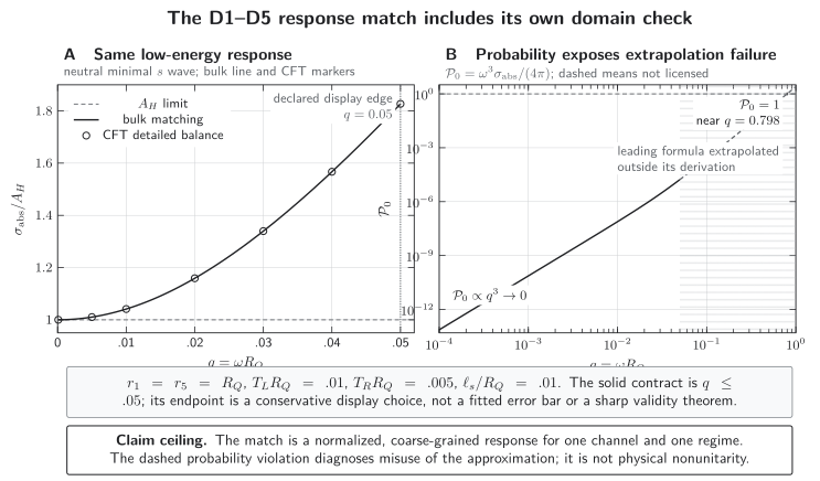
Computed benchmark for a neutral minimal $s$-wave with $r_1=r_5=R_Q$, $T_LR_Q=0.01$, $T_RR_Q=0.005$, and $\ell_s/R_Q=0.01$. In panel A, the independently evaluated bulk curve and open CFT markers coincide and approach $\sigma_{\rm abs}/A_H=1$ as $q=\omega R_Q\to0$. In panel B, $\mathcal P_0$ vanishes as $q^3$ in the declared low-energy window. The solid curve stops at the declared display boundary $q=0.05$; the dashed continuation is a deliberately invalid extrapolation of the leading low-energy formula. Its crossing of $\mathcal P_0=1$ near $q=0.798$ diagnoses loss of the approximation, not physical nonunitarity and not an uncertainty band.

The plotted values and semantic contract are available as CSV and JSON. Three checkpoints summarize the relation:

D1–D5 minimal-scalar response checkpoints for the declared numerical fixture

Checkpoint	σabs/AH	𝒫0	Interpretation
q → 0	1	0 as q3	Area law and vanishing transmission probability are compatible.
q = 0.05	1.827015241	1.6904923 × 10−5	Last point in the declared conservative display window.
q = 1	not licensed	2.4674011 from the dashed formula	𝒫0 > 1 proves that this extrapolation cannot be physical.

The bulk and CFT columns are evaluated through separate code paths, but they are algebraically equivalent representations. Their floating-point residual is an implementation and detailed-balance identity check, not independent physical evidence.

The small-$q$ expansion makes the first row analytic:

$$\frac{\sigma_{\rm abs}}{A_H} =1+\frac{q^2}{48t_Lt_R}+O(q^4), \qquad \mathcal P_0 =\frac{\widehat A_H}{4\pi}q^3+O(q^5).$$

What the thermal answer averages

The factorized thermal-line correlator is an effective continuum response. At finite circle radius $R_y$, an individual D1–D5 microstate has discrete twist-sector levels and, at sufficiently fine energy resolution, absorption lines and recurrences rather than an exactly smooth thermal spectrum. Replacing the sums by a continuum therefore requires a large-charge or long-string limit together with a probe whose energy width cannot resolve the relevant line spacing.

This distinction is observable, not philosophical. In the finite-$R_y$ two-charge D1–D5 orbifold laboratory, an incoherent beam of width $\Delta E$ gives a microstate-independent semiclassical response when $R_y\Delta E\gg1$; at finer resolution the answer depends on the microstate Das and Mandal 2009, §§1 and 4. That result is not a derivation of the present three-charge thermal formula for every state. It demonstrates why the ensemble, observation time, and resolution belong in the response contract.

Accordingly, the matched curve establishes a coarse-grained near-extremal response for the selected channel. It does not establish that every individual microstate has a horizon, an exactly thermal continuum, or the same fine-grained line spectrum. The next page on typicality and non-BPS evidence asks what would be required to promote such averaged successes to statements about overwhelmingly many states.

Adversarial tests of the match

Raise the frequency

The first failed hypothesis is the near/far overlap, not unitarity. Three controls should be separated. When $\omega r_1$ or $\omega r_5$ reaches order one, omitted terms in the matched low-frequency radial problem compete with the retained ones even if the external quantum is still soft on the string scale. When $\alpha'\omega^2$ reaches order one, string-scale excitations and higher-derivative frequency corrections enter. Independently, if $r_i^2/\alpha'$ is not large or string loops are unsuppressed, the two-derivative semiclassical background itself is uncontrolled. The dashed curve in the figure deliberately continues only the leading low-energy formula until $\mathcal P_0>1$. That impossible result diagnoses departure from its derivation. The low-energy agreement survives; an all-frequency prediction does not.

Change the polarization or angular momentum

A fixed scalar couples to charge-supported background fields and obeys a different radial equation. Its CFT dual and interaction vertex are also different; one cannot insert it into the minimal $(1,1)$ formula. Separate fixed-scalar calculations can and do match in stated regimes after the operator and normalization problem is solved Callan et al. 1997, §§4–5, especially eqs. (70), (81), and (85), David, Mandal, and Wadia 1999, §§2.3–4. The control therefore rejects formula transfer, not the D-brane description itself. Likewise, $\ell>0$ requires a new partial-wave normalization and a different CFT operator.

The historical general-charge calculation shows why the qualification matters. For unequal D1 and D5 charges, the two fixed scalars mix in the semiclassical perturbation equations. In the then-standard effective-string action, extra $(3,1)$ and $(1,3)$ chiral couplings produced a different low-energy frequency and temperature dependence, so the D-brane and semiclassical cross sections did not generally agree Taylor-Robinson 1997, §§I–IV. This is a model-dependent failure of that effective vertex under changed charge and mixing assumptions, not a failure of the correctly normalized minimal-scalar match. The strongest surviving rule is channel-by-channel: identify the physical eigenmode, its CFT operator, and its normalization before testing agreement.

Move through moduli space

The twenty minimal-scalar operators are top components of short $\mathcal N=(4,4)$ multiplets and correspond to exactly marginal directions. Their canonically normalized physical absorption cross section remains unchanged across the twenty-dimensional near-horizon moduli space: the CFT two-point, or Zamolodchikov, metric equals the metric in the bulk moduli kinetic term, so the bulk fluctuation propagator in that coordinate basis carries the inverse metric; after canonical normalization no extra coupling factor appears David, Mandal, and Wadia 2000, §5.2, eqs. (55)–(60). This is a concrete protection statement for the selected channel, not a claim that arbitrary finite-temperature correlators are coupling independent.

It is still not a BPS index theorem for arbitrary real-time dynamics. Generic operators outside the protected short-multiplet data can mix and renormalize away from the orbifold point; explicit D1–D5 conformal-perturbation calculations exhibit operator mixing that implies anomalous dimensions once the mixing matrix is completed and diagonalized Burrington, Peet, and Zadeh 2013, §§4.3–4.4 and §5. For such operators, agreement at one coupling does not license extrapolation to the supergravity regime without a separate nonrenormalization argument or a calculation along the deformation.

Common pitfalls

Calling the flux ratio a cross section. The horizon-to-infinity flux ratio is $\mathcal P_0$. In four noncompact spatial dimensions, $\sigma_{\rm abs}=(4\pi/\omega^3)\mathcal P_0$. The two quantities even have different dimensions and different low-frequency limits.

Using a proportional CFT correlator as an absolute prediction. Conformal symmetry fixes the thermal shape for a normalized $(1,1)$ operator. The prefactor also needs the canonical bulk field, $C_{\mathcal O}$, and the interaction coefficient $\mu$.

Treating stimulated absorption as the classical answer. The classical cross section is net absorption: gross absorption minus the reverse emission process. Omitting the subtraction loses the numerator $e^{\omega/T_H}-1$.

Reading a channel-specific match as a typicality theorem. The result concerns a selected operator and a coarse-grained near-extremal ensemble. Fine-resolution individual-state response is a different observable.

Exercises

1. Temperatures and the area law

Starting from the definitions of $T_L$ and $T_R$, derive $2/T_H=1/T_L+1/T_R$. Then take $\omega\to0$ in $\sigma_{\rm abs}$ and show that it equals $A_H$.

Solution

The reciprocal temperatures are

$$\frac1{T_L}=\frac{2\pi r_1r_5e^{-\delta_p}}{r_0}, \qquad \frac1{T_R}=\frac{2\pi r_1r_5e^{\delta_p}}{r_0}.$$

Their half-sum is $2\pi r_1r_5\cosh\delta_p/r_0=1/T_H$. Expanding $e^z-1=z+O(z^2)$ gives

$$\sigma_{\rm abs}(0) =4\pi^3r_1^2r_5^2\frac{T_LT_R}{T_H}.$$

Since $T_LT_R=r_0^2/(4\pi^2r_1^2r_5^2)$ and $T_H=r_0/(2\pi r_1r_5\cosh\delta_p)$, this becomes

$$\sigma_{\rm abs}(0) =2\pi^2r_0r_1r_5\cosh\delta_p=A_H.$$

2. Net absorption from detailed balance

Prove

$$(1+b_L)(1+b_R)-b_Lb_R =1+b_L+b_R =\frac{b_Lb_R}{b_H}.$$

Explain the subtraction physically.

Solution

Let $x=e^{\omega/(2T_L)}$ and $y=e^{\omega/(2T_R)}$. Then $b_L=1/(x-1)$, $b_R=1/(y-1)$, and, because $xy=e^{\omega/T_H}$, $b_H=1/(xy-1)$. Therefore

$$1+b_L+b_R =\frac{xy-1}{(x-1)(y-1)} =\frac{b_Lb_R}{b_H}.$$

The factor $(1+b_L)(1+b_R)$ counts creation of the two final CFT excitations, including Bose enhancement. The factor $b_Lb_R$ counts the reverse annihilation process. A classical incident wave measures their difference, so the absorption cross section is a net rate.

3. Cross section, probability, and phase space

Use $d^4k=2\pi^2\omega^3d\omega$ to derive

$$\frac{d\Gamma_{\rm em}}{d\omega} =\frac{\omega^3}{8\pi^2}\sigma_{\rm abs}b_H.$$

Check the dimensions of $\sigma_{\rm abs}$, $\mathcal P_0$, and $d\Gamma_{\rm em}/d\omega$.

Solution

Insert the four-dimensional spherical measure into

$$d\Gamma_{\rm em}=\sigma_{\rm abs}b_H\frac{d^4k}{(2\pi)^4}.$$

Because $2\pi^2/(2\pi)^4=1/(8\pi^2)$, the stated result follows. In natural units, $[\sigma_{\rm abs}]=L^3$, $[\omega^3]=L^{-3}$, and $[b_H]=1$, so $[d\Gamma/d\omega]=1$. This is correct because both $\Gamma$ and $\omega$ have dimension $L^{-1}$. The flux ratio $\mathcal P_0$ is dimensionless, consistent with $\mathcal P_0=\omega^3\sigma_{\rm abs}/(4\pi)$.

4. Reproduce the benchmark endpoint

For $t_L=0.01$, $t_R=0.005$, and $q=0.05$, evaluate $\sigma_{\rm abs}/A_H$ and $\mathcal P_0$. Why does the point remain inside the declared low-frequency window even though $\sigma_{\rm abs}/A_H$ is not close to one?

Solution

Use $t_H=1/150$ and

$$\frac{\sigma_{\rm abs}}{A_H} =\frac{q}{2(t_L+t_R)} \frac{e^{q/t_H}-1} {(e^{q/(2t_L)}-1)(e^{q/(2t_R)}-1)}.$$

Stable evaluation with expm1 gives

$$\frac{\sigma_{\rm abs}}{A_H}=1.827015241, \qquad \mathcal P_0=1.6904923\times10^{-5}.$$

The approximation expands in $q=\omega R_Q$, not in $\omega/T_L$ or $\omega/T_R$. Here $q=0.05\ll1$, so the wavelength remains large compared with $R_Q$ even while the frequency probes the thermal structure. This checks the frequency expansion; loop suppression remains a separate semiclassical assumption.

5. Resolve a finite-volume microstate

Suppose a twist sector behaves as a component string of length $2\pi nR_y$. Estimate its energy spacing. What condition on a probe width $\Delta E$ hides this discreteness, and why does that condition not prove typicality?

Solution

The momentum spacing is of order

$$\delta E_n\sim\frac{1}{nR_y}.$$

A probe with $\Delta E\gg\delta E_n$ averages over many neighboring lines in that sector. A stronger condition such as $R_y\Delta E\gg1$ makes even the short-component discreteness invisible and yields the broad semiclassical response in the finite-$R_y$ orbifold analysis.

This is a statement about experimental resolution. Typicality would require a measure on states and control of the fraction whose response obeys the claimed approximation. Coarse graining one state, or averaging an ensemble, does not supply that measure by itself.

What the dynamical match establishes

For one neutral minimal scalar, one near-extremal D1–D5–P ensemble, and one declared dilute-gas, low-energy regime with semiclassical control assumed, the bulk radial problem and the normalized CFT two-point function reproduce the same frequency-dependent net absorption cross section. Detailed balance then reproduces the same emission kernel. The horizon-area limit, dimensions, positivity, and deliberate extrapolation failure are physical checks; the tiny bulk/CFT numerical residual checks the implementation of an algebraic identity rather than supplying separate physical evidence.

This is real evidence for the D1–D5 operator dictionary beyond entropy counting. Its strongest licensed conclusion remains channel-specific and coarse-grained. It neither derives the Hawking state, proves an all-frequency S-matrix, nor shows that individual typical non-BPS microstates have an exactly thermal continuum. The preceding microstate-geometry page asks which states admit controlled geometric representatives; the next page asks whether protected and averaged successes extend to typical non-BPS black holes.

The chapter overview contains the structure diagram and validity and failure diagram. They are embedded there once so that their shared chapter-level context is not repeated on every article.

For the chapter-wide comparison of assumptions, counterevidence, falsifiers, and claim ceilings, see the claim-domain table.

References

• Burrington, Benjamin A., Amanda W. Peet, and Ida G. Zadeh. “Operator Mixing for String States in the D1–D5 CFT near the Orbifold Point.” Physical Review D 87, 106001 (2013). DOI. Open PDF.
• Callan, Curtis G., Steven S. Gubser, Igor R. Klebanov, and Arkady A. Tseytlin. “Absorption of Fixed Scalars and the D-Brane Approach to Black Holes.” Nuclear Physics B 489, 65–94 (1997). DOI. Open PDF.
• Das, Sumit R., Gary W. Gibbons, and Samir D. Mathur. “Universality of Low Energy Absorption Cross Sections for Black Holes.” Physical Review Letters 78, 417–419 (1997). DOI. Open PDF.
• Das, Sumit R., and Gautam Mandal. “Microstate Dependence of Scattering from the D1–D5 System.” Journal of High Energy Physics 04 (2009): 036. DOI. Open PDF.
• Das, Sumit R., and Samir D. Mathur. “Comparing Decay Rates for Black Holes and D-Branes.” Nuclear Physics B 478, 561–576 (1996). DOI. Open PDF.
• David, Justin R., Gautam Mandal, and Spenta R. Wadia. “Absorption and Hawking Radiation of Minimal and Fixed Scalars, and AdS/CFT Correspondence.” Nuclear Physics B 544, 590–611 (1999). DOI. Open PDF.
• David, Justin R., Gautam Mandal, and Spenta R. Wadia. “D1/D5 Moduli in SCFT and Gauge Theory, and Hawking Radiation.” Nuclear Physics B 564, 103–127 (2000). DOI. Open PDF.
• Maldacena, Juan M., and Andrew Strominger. “Black Hole Greybody Factors and D-Brane Spectroscopy.” Physical Review D 55, 861–870 (1997). DOI. Open PDF.
• Taylor-Robinson, Marika. “Absorption of Fixed Scalars.” arXiv:hep-th/9704172 [hep-th] (1997). Abstract. Open PDF.