Supersymmetric Localization Tests of the Quantum Entropy Function

Supersymmetric localization has produced one of the sharpest quantitative tests of black-hole microstate counting: in a restricted off-shell supergravity calculation, an infinite-dimensional near-horizon path integral becomes an ordinary integral whose Bessel-function dependence matches a microscopic Rademacher term. That statement is both remarkable and conditional. The supercharge must preserve the actual AdS₂ integration domain, the measure and contour must be controlled, every flat direction must be integrated, and the relevant saddles must be included. These conditions are not presently established for the full quantum entropy function with standard normalizable fields.

Required background. Localization Loci, Zero Modes, and One-Loop Determinants supplies the finite-dimensional localization argument; Higher-Derivative and Quantum Entropy Corrections supplies the fixed-charge correction and zero-mode bookkeeping used here.

Helpful background. Gauge Fixing and the Localization Deformation Complex explains the BRST-completed complex; AdS2 Boundary Conditions and Fragmentation explains why the AdS₂ boundary condition is part of the observable.

The fixed-charge AdS₂ observable

For electric charges $q_i$ and magnetic fluxes $p^i$, Sen’s quantum entropy function is the finite part of a Euclidean AdS₂ path integral with a boundary Wilson line,

$$d_{\rm hor}(q,p) = \left\langle \exp\!\left[-iq_i\oint_{\partial AdS_2}A^i\right] \right\rangle_{AdS_2,p}^{\rm finite}.$$

The dominant electric-field mode grows toward the AdS₂ boundary and is held fixed; Gauss’s law therefore fixes the electric charge. The constant boundary-potential mode is allowed to fluctuate, and the Wilson line makes the variational problem appropriate to that fixed-charge ensemble. The superscript “finite” means that the boundary-length divergence has been removed before the cutoff is taken away. These points are derived in Sen 2009, § 1, eq. (1.3), pp. 3–4, and § 3, eqs. (3.16)–(3.18), pp. 9–10, Open PDF.

The quantity above is a horizon partition function. Its logarithm is a quantum horizon entropy, but $d_{\rm hor}$ is not automatically an asymptotic absolute degeneracy. A microscopic comparison must specify whether the protected observable is a degeneracy or an index, remove or account for exterior hair, select the same charge orbit and single-center sector, and use the same chamber. BPS Indices, Absolute Degeneracies, and Wall Crossing explains the protected trace; the microscopic comparison contract owns the complete translation.

Charge normalizations also matter. Sen’s convention is used in the displayed definition. In the off-shell formulas below, the Dabholkar–Gomes–Murthy convention obeys $q_I^{\rm DGM}=-2q_I^{\rm Sen}$, so its Wilson insertion and the term $-\pi q_I\phi^I$ must be read with that map rather than compared symbol by symbol Dabholkar, Gomes, and Murthy 2011, § 5.3, eq. (5.33), p. 25, Open PDF.

The deformation argument and its closure gate

The historical off-shell construction chooses a fermionic symmetry $Q$ for which, up to normalization and gauge transformations,

$$Q=G_{+}^{++}+G_{-}^{--}, \qquad Q^2=4(L-J).$$

Here $L-J$ generates a compact Euclidean $U(1)$ acting simultaneously on AdS₂ and $S^2$. Gauge fixing replaces $Q$ by a compatible BRST-completed operator $\widehat Q$. For an integration cycle $\Gamma$ and a $\widehat Q$-exact deformation,

$$Z(t)=\int_{\Gamma}\!\mathcal D\Phi\, \mathcal O\, e^{-S-t\widehat QV},$$

the usual proof tries to write

$$\frac{dZ}{dt} =- \int_{\Gamma}\!\mathcal D\Phi\, \widehat Q\!\left(V\mathcal Oe^{-S-t\widehat QV}\right) =0.$$

The last equality is not algebra alone. It is an integration-by-parts statement on field space. It requires all of the following:

Gate	What must be checked
Domain closure	$\widehat Q$ maps every allowed field and ghost fluctuation back into the same boundary-condition and normalizability class.
Compact square	$\widehat Q^2$ generates a compact bosonic symmetry, modulo gauge transformations treated by the same complex.
Invariant data	The action, insertion, regulator, measure, and contour are invariant under $\widehat Q$.
No boundary flux	The total derivative has no contribution from infinity in spacetime, infinity or singular strata in field space, or a contour endpoint.
Complete zero-mode treatment	The kernel and cokernel of the deformation complex are identified and their collective coordinates are integrated with the induced measure.

The first gate fails for the standard continuum of delta-normalizable AdS₂ modes in the presently known construction. At large radial coordinate $\eta$, a typical mode and a Killing spinor behave as

$$f_\lambda\sim e^{-\eta/2}e^{\pm i\lambda\eta}, \qquad \epsilon\sim e^{\eta/2},$$

so their supersymmetry variation has the asymptotic size

$$\delta_\epsilon f_\lambda \sim e^{\pm i\lambda\eta}.$$

It no longer belongs to the original delta-normalizable space. A BRST completion does not by itself repair this mismatch, because the independently integrated fields must still remain inside their declared domains. Sen also finds additional kernel–cokernel mismatches and cutoff-sensitive finite terms. Consequently, the familiar $dZ/dt=0$ step is a conditional formal identity for the full standard QEF, not a completed theorem Sen 2026, §§ 2–5 and § 8, especially eqs. (3.1)–(3.5) and (3.16)–(3.20), Open PDF.

There is a useful positive result inside the obstruction. The metric and gravitino zero-mode subsector closes under the relevant super-Virasoro algebra and localizes to the compact space $SU(2)/U(1)\simeq S^2$; its net dependence on the common near-horizon radius $a$ is $a^0$, so this sector contributes no power of the horizon scale. This does not localize the gauge zero modes or the full continuum, but it shows that a carefully isolated closed sector can still be treated exactly Sen 2026, §§ 6–7, especially eqs. (6.18)–(6.20) and (7.6)–(7.10), Open PDF.

The off-shell vector-multiplet branch

Subject to the closure gate, the classic calculation uses four-dimensional off-shell $\mathcal N=2$ conformal supergravity. On the vector-multiplet/F-term branch, constants $C^I$ label coordinate-dependent profiles rather than constant fields. With $r=\cosh\eta$,

$$X^I(r)=X_*^I+\frac{C^I}{r}, \qquad \bar X^I(r)=\bar X_*^I+\frac{C^I}{r},$$ $$Y^{I1}{}_{1}=-Y^{I2}{}_{2}=\frac{2C^I}{r^2}, \qquad X_*^I=\frac{e_*^I+ip^I}{2}, \qquad \phi^I=e_*^I+2C^I.$$

The metric, gauge fields, and the remaining Weyl-multiplet fields stay on their attractor values on this branch. The falloff $C^I/r$ is normalizable, while the center value $\phi^I$ becomes a collective coordinate. These profiles and their renormalized action are derived in Dabholkar, Gomes, and Murthy 2011, § 5.3, eqs. (5.30)–(5.32) and (5.48)–(5.52), pp. 24–30, Open PDF.

Let $F(X,\widehat A)$ be the homogeneous holomorphic function encoding the retained F-type couplings,

$$F(\lambda X,\lambda^2\widehat A) =\lambda^2F(X,\widehat A).$$

Here $\widehat A$ is the lowest scalar in the chiral multiplet built from the square of the Weyl multiplet; $\widehat A_\ast$ and $\bar{\widehat A}_\ast$ below are its fixed attractor-background values.

On the real collective-coordinate slice, the renormalized action is

$$\mathcal S_{\rm loc}(\phi;q,p) =-\pi q_I\phi^I+\mathcal F(\phi,p),$$

where

$$\mathcal F(\phi,p) =-2\pi i\!\left[ F\!\left(\frac{\phi^I+ip^I}{2},\widehat A_\ast\right) - \bar F\!\left(\frac{\phi^I-ip^I}{2},\bar{\widehat A}_\ast\right) \right].$$

On that real slice, $\mathcal F=4\pi\operatorname{Im}F$. After complexifying the contour, however, “take the imaginary part” is not an analytic prescription: the north- and south-pole branches must be continued separately.

The restricted smooth-saddle contribution therefore has the schematic form

$$\widehat W_0(q,p) = \int_{\mathcal C}[d\phi]_\mu\, Z_{\rm det}(\phi,p)\, Z_{\rm inst}^{N}(\phi,p) Z_{\rm anti}^{S}(\phi,p)\, e^{\mathcal S_{\rm loc}(\phi;q,p)}.$$

This is not an equation for the full string path integral. The measure, one-loop determinant, contour, polar instanton factors, omitted multiplets, non-F-type interactions, other localizing branches, and other gravitational saddles remain additional inputs. Gupta and Murthy found a more general off-shell solution space when the auxiliary $SU(2)$ curvature is allowed to fluctuate, and the 2026 kernel analysis exposes further flat directions Gupta and Murthy 2013, abstract and §§ 4–5, Open PDF. The separate polar instanton factors should also not double-count worldsheet-instanton corrections already present in $F$.

Worked test: one-eighth-BPS dyons in N=8 theory

The cleanest worked charge family is type II string theory on $T^6$. Select the five-charge one-eighth-BPS orbit

$$\Gamma(n,\nu) = \begin{pmatrix} 0&n&0&1\\ 1&\nu&1&0 \end{pmatrix}, \qquad \nu\in\{0,1\}, \qquad \Delta=4n-\nu^2>0.$$

Here $\Delta=Q^2P^2-(Q\mathbin{\cdot}P)^2$ is the quartic invariant of the continuous duality group $E_{7,7}(\mathbb R)$ in this frame. The charge family represents a selected arithmetic $E_{7,7}(\mathbb Z)$ orbit; not every charge vector with the same $\Delta$ is necessarily related to it by the discrete duality group.

A one-eighth-BPS state preserves four of the 32 supercharges and breaks 28, producing 14 fermion-zero-mode pairs. The zero-mode-saturated asymptotic invariant is the four-dimensional helicity trace

$$B_{14}(\Gamma) =\frac{1}{14!} \operatorname{Tr}_{\Gamma}\!\left[ (-1)^{2J_3}(2J_3)^{14} \right].$$

For the D-brane charge frame used here, the positive integer compared with the horizon QEF is

$$d(\Delta)\equiv -B_{14}(\Gamma)$$

after removing the exterior-hair contribution. This identification assumes that the only relevant exterior modes are the broken-supersymmetry fermion zero modes; if additional hair is present, its index must be divided out separately. BPS Indices, Absolute Degeneracies, and Wall Crossing develops that distinction, while Sen 2010, § 1, pp. 1–2, Open PDF fixes the $-B_{14}$ convention for this $\mathcal N=8$ charge sector.

Using the Dabholkar–Gomes–Murthy theta convention,

$$\vartheta_1(\tau,z) =q_\tau^{1/8}(y^{1/2}-y^{-1/2}) \prod_{k=1}^{\infty} (1-q_\tau^k)(1-yq_\tau^k)(1-y^{-1}q_\tau^k),$$

the protected coefficients are defined by

$$\frac{\vartheta_1(\tau,z)^2}{\eta(\tau)^6} =\sum_{\substack{m\ge0\\ r\in\mathbb Z}} C(4m-r^2)q_\tau^m y^r, \qquad q_\tau=e^{2\pi i\tau}, \quad y=e^{2\pi iz},$$

where $q_\tau$ is the modular nome and $y$ is the elliptic fugacity; $q_\tau$ is unrelated to the electric charges $q_I$. This convention fixes the otherwise ambiguous overall sign of the Fourier coefficients Dabholkar, Gomes, and Murthy 2013, § 3.2, eqs. (3.12)–(3.16), pp. 7–8, Open PDF. The sign-corrected positive coefficients in this orbit are

$$d(\Delta)=(-1)^{\Delta+1}C(\Delta).$$

The microscopic derivation can be organized in a D1–D5 frame with a Kaluza–Klein monopole; D1–D5 CFT and AdS3 Microstate Data supplies the broader brane/CFT setting. Here only the protected Fourier coefficient and its precise charge orbit are used.

The exact microscopic Rademacher series is most transparent in terms of the normalized Bessel integral

$$\widetilde I_\rho(z) =\frac{1}{2\pi i} \int_{\epsilon-i\infty}^{\epsilon+i\infty} \frac{d\sigma}{\sigma^{\rho+1}} \exp\!\left(\sigma+\frac{z^2}{4\sigma}\right) =\left(\frac z2\right)^{-\rho}I_\rho^{\rm std}(z), \qquad \epsilon>0.$$

In these conventions,

$$C(\Delta) =2\pi\left(\frac{\pi}{2}\right)^{7/2} \sum_{c=1}^{\infty} c^{-9/2}K_c(\Delta) \widetilde I_{7/2}\!\left(\frac{\pi\sqrt\Delta}{c}\right),$$

and

$$K_1(\Delta)=\frac{(-1)^{\Delta+1}}{\sqrt2}.$$

This side of the comparison is a mathematical identity for the stated Fourier coefficients Dabholkar, Gomes, and Murthy 2013, § 3.2 and § 3.4, eqs. (3.12) and (3.33)–(3.41), pp. 7–12, Open PDF.

On the conditional macroscopic side, the $\mathcal N=2$ truncation has $n_v=7$ physical vector multiplets, with the compensating vector giving indices $I=0,\ldots,7$. After the proposed induced measure, Gaussian integrations, and analytic continuation of the wrong-sign conformal mode, the smooth $c=1$ sector reduces to

$$\widehat W_1(\Delta) \propto \int_{\operatorname{Re}\sigma=\epsilon>0} \frac{d\sigma}{\sigma^{9/2}} \exp\!\left( \sigma+\frac{\pi^2\Delta}{4\sigma} \right) \propto \widetilde I_{7/2}(\pi\sqrt\Delta).$$

After fixing one overall constant to the microscopic normalization, the resulting $c=1$ function can be written with the standard modified Bessel function as

$$W_1(\Delta) =\sqrt2\,\pi\,\Delta^{-7/4} I_{7/2}^{\rm std}(\pi\sqrt\Delta).$$

This predicts nontrivial charge dependence, not a first-principles absolute normalization. Since

$$I_\rho^{\rm std}(z) \sim\frac{e^z}{\sqrt{2\pi z}} \left[1-\frac{4\rho^2-1}{8z}+O(z^{-2})\right],$$

the localized $c=1$ function has

$$\log W_1(\Delta) =\pi\sqrt\Delta-2\log\Delta+O(1)+O(\Delta^{-1/2}).$$

The $-2\log\Delta$ is easy to trace: $\Delta^{-7/4}$ supplies $-7\log\Delta/4$, while $z^{-1/2}$ with $z=\pi\sqrt\Delta$ supplies the remaining $-\log\Delta/4$.

The finite-charge comparison is striking:

$\Delta$	Exact microscopic $d(\Delta)$	Normalized $c=1$ term $W_1(\Delta)$	Area-law exponential $e^{\pi\sqrt\Delta}$
$3$	$8$	$7.97155\ldots$	$230.765\ldots$
$4$	$12$	$12.20123\ldots$	$535.492\ldots$
$12$	$208$	$208.45493\ldots$	$53252.3\ldots$

The values of $W_1$ follow independently from the displayed standard-Bessel formula and agree with Dabholkar, Gomes, and Murthy 2013, § 5.3, eqs. (5.28)–(5.30) and Table 2, pp. 23–24, Open PDF. The small difference between $d$ and $W_1$ is supplied by the $c>1$ Rademacher images. The proximity at small $\Delta$ is illustrative; semiclassical supergravity is controlled only at large charge, and the gravitational derivation remains subject to the closure gate.

The figure now collects the logical order. Read the solid route as a conditional calculation: every step to the right is licensed only after the closure gate. The dashed route is an explicit failed control, not another saddle.

On a narrow screen, swipe or use the Left and Right arrow keys to pan across the figure. Home and End move to its edges. A full-size link is also available.

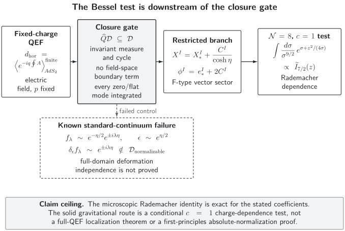
The solid route is the historical conditional calculation: the fixed-charge QEF, after successful domain, measure, contour, and zero-mode gates, is restricted to an off-shell vector-multiplet branch and then to the $\mathcal N=8$ integral that reproduces the $c=1$ Rademacher Bessel dependence. The dashed control shows the known obstruction for standard continuum modes: multiplying their $e^{-\eta/2}$ falloff by a Killing spinor growing as $e^{\eta/2}$ produces a non-normalizable variation, so deformation independence of the full QEF has not been proved. The diagram is schematic and not a count of degrees of freedom.

Orbifold sectors and the nonperturbative tail

The $c>1$ terms are exponentially smaller than the leading image because their Bessel argument is $\pi\sqrt\Delta/c$. A proposed macroscopic realization uses freely acting supersymmetric quotients combining opposite rotations of AdS₂ and $S^2$ with an internal shift. In a simple frame,

$$(\widetilde\theta,\widetilde\varphi,\widetilde y) \sim \left( \widetilde\theta+\frac{2\pi}{c}, \widetilde\varphi-\frac{2\pi}{c}, \widetilde y+\frac{2\pi\delta}{c} \right), \qquad \gcd(c,\delta)=1.$$

The renormalized action is divided by $c$, producing the Bessel argument $\pi\sqrt\Delta/c$. Boundary Wilson lines and gauge and gravitational Chern–Simons terms supply arithmetic phases. The 2013 analysis showed that exact agreement would require the remaining factor to equal $c^{-9/2}K_c(\Delta)$; the 2015 analysis derived the charge-dependent Kloosterman phases for specified orbifold saddles. It did not establish every determinant, normalization, level shift, or the completeness of the saddle set Dabholkar, Gomes, and Murthy 2013, § 5.4, eqs. (5.31)–(5.41), pp. 25–27, Open PDF; Dabholkar, Gomes, and Murthy 2015, §§ 3–5, especially eqs. (5.23)–(5.26), Open PDF.

Every candidate quotient must separately pass flux quantization, spin-structure, smoothness, supersymmetry, boundary-condition, and arithmetic divisibility checks. “Include the orbifolds” is not a substitute for specifying that set.

What is established and what remains conditional

The following separation is the scientific conclusion, not merely a list of technical details.

Ingredient	Current status	Consequence for a claim
Fixed-charge Wilson-line QEF	Defined with explicit AdS₂ boundary conditions and finite-part prescription	The horizon observable and ensemble are well specified.
Restricted F-term profiles and action	Derived off shell on the stated vector-multiplet branch	The finite collective-coordinate integrand is meaningful within that truncation.
Microscopic Rademacher expansion	Exact for the stated Jacobi-form coefficients	Bessel orders, arithmetic phases, and integer coefficients provide sharp targets.
Selected vector/hyper determinants	Computed for stated gauges and regulators, but not all multiplets	They test pieces of the measure; they do not complete the full QEF.
Standard QEF domain under $Q$	Not closed for generic delta-normalizable modes in the known construction	Deformation independence of the full standard-domain integral is unproved.
Complete locus and flat directions	Additional modes remain beyond the familiar $C^I$ branch	Unidentified integrals cannot be replaced by a unit factor.
Measure and UV regulator	No first-principles UV-complete prescription; finite charge-ratio terms can move	Absolute coefficients and $O(1)$ terms require a claim downgrade.
Contour	Analytic continuation is required and pole or Stokes crossings can change the answer	The cycle is physical data, not a cosmetic convergence choice.
Orbifold saddle sum	Bessel arguments and selected phases are understood; completeness and determinants are not	The all-$c$ equality remains conditional.
Microscopic interpretation	Depends on index, hair, chamber, charge orbit, and center selection	Agreement cannot be promoted automatically to an absolute all-state count.

For example, vector- and hypermultiplet deformation determinants have been computed under specified assumptions, while the Weyl, gravitino, and full measure problem remain incomplete Murthy and Reys 2015, § 4, eqs. (4.27)–(4.28), and § 6, Open PDF; Gupta, Ito, and Jeon 2015, § 5, eq. (5.18), and § 6, Open PDF. A zero $\widehat Q$-index or a charge-independent determinant in one sector does not license deleting the other sectors.

As of August 29, 2026, the defensible evidence ceiling is therefore: a historically important conditional finite-dimensional supergravity calculation reproduces the $c=1$ microscopic Bessel dependence and parts of the nonperturbative arithmetic structure; a restricted metric/gravitino zero-mode subsector localizes securely. It is not yet an exact evaluation of the full physical QEF.

Adversarial tests and stop rules

An exactness claim should survive all five controls below.

Vary the measure. Replace

$$\frac{d\sigma}{\sigma^{9/2}} \longrightarrow \frac{d\sigma}{\sigma^{9/2-\alpha}}.$$

The normalized Bessel order becomes $7/2-\alpha$. If no other factor compensates, the logarithmic coefficient moves from $-2$ to $-2+\alpha/2$. Thus an unproved zero-mode Jacobian changes precisely the subleading data used as the test.

Move the contour. The conformal compensator requires analytic continuation to a Bromwich-type cycle with $\operatorname{Re}\sigma>0$. Crossing $\sigma=0$, a pole of an instanton factor, or a Stokes wall can add residues or change the saddle decomposition. Until the homologous cycle is fixed, report contour-dependent alternatives rather than a unique number.

Omit allowed saddles. Keeping only $c=1$ preserves every power correction around $e^{\pi\sqrt\Delta}$ but misses an absolute correction beginning at order $e^{\pi\sqrt\Delta/2}$ when an allowed $c=2$ sector is present. That error is relatively $e^{-\pi\sqrt\Delta/2}$, yet it remains visible in exact integer coefficients.

Test domain closure. Act with $\widehat Q$ on a complete basis of allowed continuum and zero modes. A single transformed mode outside the boundary-condition space blocks the field-space integration by parts and therefore blocks the full localization claim. The explicit $e^{-\eta/2}\times e^{\eta/2}$ control already fails for the standard continuum.

Count every flat direction. Determine the kernel and cokernel of the deformation complex and integrate the residual coordinates. Sen finds an index mismatch for the $\mathcal N=2$ graviton multiplet and for each omitted gravitino multiplet. Assigning the unexplained modes a determinant of one would assume the result that the measure calculation is meant to establish Sen 2026, § 4 and § 8, Open PDF.

Stop at the first failed control. The strongest surviving statement may still be valuable—for example, exact microscopic Rademacher structure, a conditional $c=1$ functional match, or localization of a closed zero-mode subsector—but its hypotheses must travel with it.

Common pitfalls

Calling the collective coordinates constant fields. The numbers $C^I$ are constant labels, but $X^I(r)$ and $Y^I(r)$ vary over AdS₂. This distinction is exactly what allows a nontrivial off-shell profile to remain in the chosen supersymmetric branch.

Using $4\pi\operatorname{Im}F$ after complexifying the contour. That expression is convenient on the real slice. A complex cycle requires separate analytic continuations of the holomorphic and antiholomorphic branches, together with a statement of which poles and Stokes sectors the cycle avoids.

Equating a Bessel match with a complete path integral. The $I_{7/2}$ dependence is exact for the displayed reduced integral and for the corresponding microscopic Rademacher image. It does not prove domain closure, absolute normalization, completeness of multiplets, or completeness of gravitational saddles.

Forgetting what was counted. The $T^6$ charge example compares a protected indexed coefficient in a selected charge orbit with a fixed-charge horizon quantity after the appropriate zero-mode and hair interpretation. Replacing either side by an unqualified absolute degeneracy changes the question.

Exercises

1. Test the supersymmetry domain

A standard delta-normalizable bosonic fluctuation behaves as $f_\lambda\sim e^{-\eta/2\pm i\lambda\eta}$, while the relevant Killing spinor behaves as $\epsilon\sim e^{\eta/2}$. Determine the asymptotic size of $\delta_\epsilon f_\lambda$, decide whether the standard field domain is closed under $Q$, and state precisely which localization inference fails.

Solution

Multiplying the radial factors gives

$$\delta_\epsilon f_\lambda \sim e^{\eta/2}e^{-\eta/2\pm i\lambda\eta} =e^{\pm i\lambda\eta}.$$

The variation no longer has the decaying factor required by the standard delta-normalizable domain, so $Q\mathcal D\not\subseteq\mathcal D$. The integration-by-parts step that would turn the $Q$-exact deformation into $dZ/dt=0$ can then acquire a field-space boundary contribution. Thus deformation independence of the full standard-domain QEF is not established, although a separately identified $Q$-closed subsector may still localize.

2. Recover the logarithmic term

Starting from

$$W_1(\Delta) =\sqrt2\,\pi\,\Delta^{-7/4} I_{7/2}^{\rm std}(\pi\sqrt\Delta),$$

use the leading large-$z$ asymptotic of $I_\rho^{\rm std}(z)$ to find the coefficient of $\log\Delta$ in $\log W_1$.

Solution

Set $z=\pi\sqrt\Delta$. Then

$$\log I_{7/2}^{\rm std}(z) =z-\frac12\log(2\pi z)+O(z^{-1}).$$

Because $\log z=\tfrac12\log\Delta+O(1)$,

$$\log W_1 =\pi\sqrt\Delta -\frac74\log\Delta -\frac14\log\Delta +O(1)+O(\Delta^{-1/2}).$$

The coefficient is therefore $-2$.

3. Detect a wrong measure

Show that replacing $d\sigma/\sigma^{9/2}$ by $d\sigma/\sigma^{9/2-\alpha}$ changes the normalized Bessel index and the logarithmic coefficient.

Solution

The defining integral has denominator $\sigma^{\rho+1}$. Therefore

$$\rho+1=\frac92-\alpha \quad\Longrightarrow\quad \rho=\frac72-\alpha.$$

At large $z$, $\widetilde I_\rho(z)\sim e^z z^{-\rho-1/2}$ up to a constant. Since $z\propto\sqrt\Delta$, the reduced integral contributes

$$\log\widetilde I_{7/2-\alpha}(\pi\sqrt\Delta) =\pi\sqrt\Delta +\left(-2+\frac\alpha2\right)\log\Delta +O(1)+O(\Delta^{-1/2}).$$

Unless another independently derived factor cancels the change, the microscopic $-2\log\Delta$ test fails for every $\alpha\ne0$.

4. Separate perturbative and nonperturbative precision

Suppose the $c=1$ term is kept but an allowed $c=2$ quotient is omitted. Which part of the large-charge expansion remains correct, and which exact claim fails?

Solution

The $c=1$ Bessel function contains the full asymptotic power series multiplying $e^{\pi\sqrt\Delta}$, so its logarithmic and inverse-charge corrections remain intact. The leading omitted quotient scales as $e^{\pi\sqrt\Delta/2}$ times powers and phases. It is exponentially small relative to $c=1$, so it does not alter the perturbative series around that saddle, but it changes the exact finite-charge coefficient. Therefore perturbative agreement survives while equality with the full microscopic integer does not.

Localization tests protected horizon data. The next article turns to a different question: whether known smooth horizonless solutions are numerous and typical enough to represent black-hole microstates. Continue to Microstate Geometries and Fuzzball Proposals.

The chapter overview contains the structure diagram and validity and failure diagram. They are embedded there once so that their shared chapter-level context is not repeated on every article.

For the chapter-wide comparison of assumptions, counterevidence, falsifiers, and claim ceilings, see the claim-domain table.

References

• Dabholkar, Atish, João Gomes, and Sameer Murthy. “Quantum Black Holes, Localization and the Topological String.” Journal of High Energy Physics 06 (2011): 019. DOI. Open PDF.
• Dabholkar, Atish, João Gomes, and Sameer Murthy. “Localization & Exact Holography.” Journal of High Energy Physics 04 (2013): 062. DOI. Open PDF.
• Dabholkar, Atish, João Gomes, and Sameer Murthy. “Nonperturbative Black Hole Entropy and Kloosterman Sums.” Journal of High Energy Physics 03 (2015): 074. DOI. Open PDF.
• Gupta, Rajesh Kumar, Yuto Ito, and Imtak Jeon. “Supersymmetric Localization for BPS Black Hole Entropy: 1-Loop Partition Function from Vector Multiplets.” Journal of High Energy Physics 11 (2015): 197. DOI. Open PDF.
• Gupta, Rajesh Kumar, and Sameer Murthy. “All Solutions of the Localization Equations for $\mathcal N=2$ Quantum Black Hole Entropy.” Journal of High Energy Physics 02 (2013): 141. DOI. Open PDF.
• Murthy, Sameer, and Valentin Reys. “Functional Determinants, Index Theorems, and Exact Quantum Black Hole Entropy.” Journal of High Energy Physics 12 (2015): 028. DOI. Open PDF.
• Sen, Ashoke. “Quantum Entropy Function from AdS2/CFT1 Correspondence.” International Journal of Modern Physics A 24, no. 23 (2009): 4225–4244. DOI. Open PDF.
• Sen, Ashoke. “Arithmetic of N=8 Black Holes.” Journal of High Energy Physics 02 (2010): 090. DOI. Open PDF.
• Sen, Ashoke. “Revisiting Localization for BPS Black Hole Entropy.” Journal of High Energy Physics 08 (2026): 174. DOI. Open-access article.