Localization Loci, Zero Modes, and One-Loop Determinants

A localized path integral is a sum or integral over the zeros of a chosen deformation in every allowed field and bundle sector. Only under suitable positivity and reality assumptions do those zeros coincide simply with the $Q$-fixed configurations. Nonzero fluctuations give a regulated superdeterminant of the gauge-fixed complex; kernel modes instead produce collective-coordinate measures, stabilizer quotients, or fermionic selection rules. Keeping these operations separate is the core of a correct one-loop formula.

Required background. Gauge fixing and the localization deformation complex supplies the graded operator whose cohomology and determinant are required. Heat kernels, zeta functions, and spectral determinants supplies spectral regularization.

Helpful background. Generalized Killing spinors and global spin-R bundles supplies flux sectors and fixed-point bundle data.

From deformation independence to the locus

Begin in a specified field-space cycle $\Gamma$ and topological sector $\nu$:

$$Z_\nu(t)=\int_{\Gamma_\nu}\mathcal D\Phi\; e^{-S[\Phi]-t\widehat QV[\Phi]}.$$

The familiar equation $dZ_\nu/dt=0$ is justified only if the measure and original action are $\widehat Q$ invariant, $\Gamma_\nu$ is preserved by $\widehat Q$, and integration by parts in field space has no contribution from a boundary or infinity. Subject to those conditions, one may take $t\to+\infty$.

On a real cycle for which

$$(\widehat QV)_{\rm bos} =\sum_a\lVert\widehat Q\Psi_a\rVert_\Gamma^2,$$

the deformation is nonnegative and its zero set obeys

$$\widehat Q\Psi_a=0$$

for every fermion $\Psi_a$. Auxiliaries must be eliminated on their declared contours, and the gauge condition must be imposed as part of the combined complex. On a complex cycle the displayed “norm” need not be positive; the relevant objects may instead be critical points or critical manifolds of a Morse function. Thus “solve $Q\Psi=0$” is a conclusion in the positive case and only a candidate saddle equation in the general complex case.

The global locus is

$$\mathcal M_Q =\bigsqcup_{\nu} \left\{\Phi:\ (\widehat QV)_{\rm bos}=0\right\}_{\nu} \big/\mathcal G_\nu.$$

The labels $\nu$ are fixed by the global gauge group and the allowed bundles, not merely by its Lie algebra. They can include magnetic flux, instanton number, discrete characteristic classes, holonomy sectors, or defect charges. A calculation in the trivial bundle is not a proof that the other components vanish. For example, the smooth bulk locus on $S^4$ is accompanied by pointlike instanton and anti-instanton sectors at the two fixed poles Pestun 2012, §§3.4 and 4.3.

Finally evaluate the undeformed action, including topological, boundary, and supersymmetric counterterms, on each component. This gives the classical weight $e^{-S_{\rm cl}(m,\nu)}$; it is not determined by the quadratic localizing term.

Deriving the collective-coordinate measure

Let $m^i$ be local coordinates on a smooth component and $\Phi_0(m)$ a family of representatives. A derivative $\partial_i\Phi_0$ generally has a gauge component. Choose $\epsilon_i$ so that

$$Z_i =\frac{\partial\Phi_0}{\partial m^i} +\delta_{\epsilon_i}\Phi_0, \qquad D_{\rm gauge}^{\dagger}Z_i=0.$$

The physical zero modes $Z_i$ have Gram matrix

$$G_{ij}(m)=\langle Z_i,Z_j\rangle.$$

Changing variables from orthonormal field modes to $m^i$ therefore contributes

$$d\mu_{\rm coll}(m) \propto \sqrt{\det G(m)}\,\prod_i dm^i.$$

The proportionality constant depends on the normalization of the ultraviolet functional measure and on whether the variables are real or complex. It cannot be recovered by putting a prime on a determinant.

The local quotient supplies further data. If $G_{\Phi_0}$ is the stabilizer, its zero modes are removed from the Faddeev–Popov determinant and replaced by the correctly normalized residual group quotient or integral. A residual Weyl-group quotient is included once, not once in gauge fixing and again in the final integral. At a reducible or singular stratum, a smooth measure $\sqrt{\det G}\,dm$ may fail; an obstruction bundle, Euler class, or a separate local model can be required.

Fermionic zero modes behave differently. If $\eta^alpha$ are Grassmann collective coordinates, the sector contains $\prod_alpha d\eta^alpha$. It vanishes unless observables or interaction terms supply every $\eta^alpha$ needed to saturate the integral.

Gaussian nonzero modes

Expand about $\Phi_0(m)$ and rescale nonzero fluctuations by $t^{-1/2}$. The quadratic action is schematically

$$S_t=S_{\rm cl}(m) +\frac12\langle x,K_Bx\rangle +\langle\bar\psi,K_F\psi\rangle +O(t^{-1/2}).$$

For finite-dimensional, positive real bosonic modes and complex Grassmann modes,

$$\int d^nx\,e^{-x^{\mathsf T}K_Bx/2} =(2\pi)^{n/2}(\det K_B)^{-1/2},$$ $$\int d^n\bar\psi\,d^n\psi\, e^{-\bar\psi K_F\psi}=\det K_F.$$

An antisymmetric quadratic form in real fermions instead gives $\operatorname{Pf}K_F$, whose square is $\det K_F$. After declaring measure normalizations, the formal nonzero-mode factor is therefore

$$Z_{\rm 1-loop} =\frac{\det'K_F}{\sqrt{\det'K_B}},$$

or the corresponding Pfaffian ratio. The prime means “restrict to the chosen complement of the kernel.” It neither integrates the kernel nor fixes a square-root or Pfaffian phase.

Supersymmetry pairs most nonzero modes. For a two-term representative $D:E_0\to E_1$, the positive operators $D^\dagger D$ and $DD^\dagger$ have identical nonzero singular values. The uncancelled multiplicities are encoded by

$$\operatorname{ind}_{\mathcal H}D =\operatorname{Tr}_{\ker D}e^{t\mathcal H} -\operatorname{Tr}_{\ker D^\dagger}e^{t\mathcal H}.$$

For a longer complex one uses its alternating equivariant cohomology. An index supplies a virtual representation of $\mathcal H$; turning its weights into an infinite product still requires an expansion convention, a regulator, and zero-weight removal. This separation is explicit in the cohomological and fixed-point analysis of five-dimensional gauge theory in Qiu and Zabzine 2017, §§3–5.

Determinant lines, phases, and regulators

For a Fredholm operator $D$, use the convention

$$\operatorname{Det}D =\det(\ker D)\otimes \det(\operatorname{coker}D)^*.$$

As background fields or collective coordinates vary, these one-dimensional spaces form a determinant line bundle. A fermion determinant or Pfaffian is naturally a section of such a line, not automatically a globally defined complex number. A phase convention is a trivialization and orientation of the relevant line; nontrivial holonomy can encode a global anomaly. The determinant-line and eta-invariant framework, including its gluing meaning, is developed in Dai and Freed 1994, §§1–3.

For a positive elliptic operator $K$ with its kernel removed, zeta regularization defines

$$\zeta_K(s)=\sum_{\lambda\ne0}\lambda^{-s}, \qquad \log\det'_{\zeta}K=-\zeta'_K(0),$$

after meromorphic continuation. A first-order or non-self-adjoint operator also needs a spectral cut to define $\lambda^{-s}$, so the cut can change the phase. Heat-kernel, zeta, Pauli–Villars, and index-character prescriptions can differ by allowed local counterterms when they preserve the same symmetries. They need not agree when one prescription hides an anomaly or chooses a different determinant-line trivialization.

Useful consistency checks include:

1. mass dimensions and renormalization-scale dependence;
2. cancellation in a free supersymmetric multiplet with a known spectrum;
3. explicit treatment when an eigenvalue crosses zero;
4. agreement between harmonic analysis and the equivariant index;
5. large-mass decoupling up to allowed local terms;
6. invariance under large gauge transformations for the declared global gauge group.

The complete schematic answer

Once all these data have been supplied, the contribution has the structure

$$Z =\sum_\nu \int_{\Gamma_\nu\subset\mathcal M_{Q,\nu}} d\mu_\nu(m)\; e^{-S_{\rm cl}(m,\nu)} Z_{{\rm 1-loop},\nu}(m) Z_{{\rm nonpert},\nu}(m).$$

$d\mu_\nu$ includes collective-coordinate Jacobians, stabilizer data, and fermionic-zero-mode saturation. $Z_{\rm nonpert}$ contains additional localized sectors, such as pointlike instantons, only after a compactification and factorization prescription has defined that separation. Without a sector list, cycle, measure, phase, and regulator, the displayed expression is a formal template rather than a defined observable.

The middle of the shared chain below organizes the ingredients hidden by that template. A complete sector-by-sector zero set must first be split into collective coordinates, stabilizers, fermionic kernels, and paired nonzero modes. Only the last group belongs in a primed determinant.

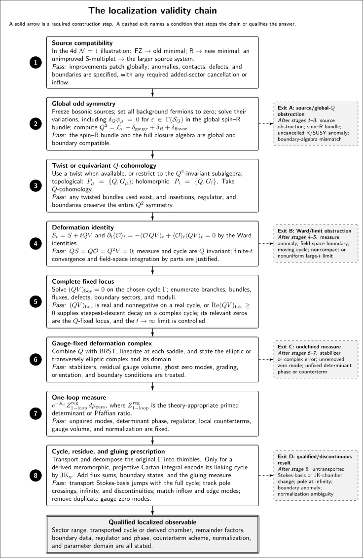
Stages five through seven separate the full zero set of $(\widehat QV)_{\rm bos}$ in every bundle and flux sector from the combined supersymmetry–BRST complex, its stabilizer and obstruction cohomology, the collective-coordinate measure, and the regulated primed determinant. The shortcut $\widehat Q\Psi=0$ is valid only on a real cycle where the bosonic deformation is a nonnegative sum of the stated squares; a complex cycle instead needs its own critical-set and steepest-descent analysis. Dashed exits flag missed sectors, nonuniform large-$t$ limits, reducible saddles, zero-mode errors, determinant-line phases, and unfixed counterterms. The full diagram is schematic and not to scale; supercharge and R-charge normalizations are theory dependent.

The reflowing text equivalent of the eight-stage chain preserves every input, construction, pass condition, output, and failure exit for narrow-screen and print reading.

Common pitfalls

A primed determinant without a replacement measure. Removing a zero eigenvalue is only half the operation. State whether it becomes a modulus, a stabilizer quotient, or a Grassmann integral.

The perturbative locus is called complete. Fluxes, reducible connections, pointlike instantons, and singular strata must be excluded by an argument or included in the sector sum.

The index is called the determinant. An index gives virtual unpaired multiplicities. It does not choose a product, regulator, determinant-line orientation, or phase.

Exercises

1. The zero-mode Jacobian. Let $Z_i$ be a basis of real bosonic zero modes and write a zero-mode fluctuation as $\delta\Phi=Z_i\,\delta m^i$. Show that the volume element inherited from the field-space metric is $\sqrt{\det G}\,\prod_i dm^i$.

Solution

The squared distance is

$$\lVert\delta\Phi\rVert^2 =\langle Z_i,Z_j\rangle dm^i dm^j =G_{ij}dm^i dm^j.$$

The Riemannian volume element of this metric is $\sqrt{\det G}\,\prod_i dm^i$. Overall powers of $2\pi$ or the coupling come from the normalization chosen for the original functional measure and must be restored from that convention.

2. Fermion zero modes. Why does a saddle with one unsaturated Grassmann zero mode contribute zero to the partition function?

Solution

The zero-mode integral contains $\int d\eta\,1=0$. A contribution requires an insertion or interaction supplying a factor of $\eta$; then $\int d\eta\,\eta=1$.

3. Singular-value cancellation. Let $D$ have nonzero singular values $s_n$. Show that

$$\frac{\det'^{1/2}(DD^\dagger)} {\det'^{1/2}(D^\dagger D)}=1$$

when the same regulator is used. What information is missing from this equality?

Solution

Both positive operators have nonzero eigenvalues $s_n^2$ with the same multiplicities, so their regulated products cancel. The equality omits the unequal kernels and cokernels, their collective-coordinate or Grassmann measures, and any phase belonging to the underlying first-order fermion operator.

References

• Dai, Xianzhe, and Daniel S. Freed. “$\eta$-Invariants and Determinant Lines.” Journal of Mathematical Physics 35, no. 10 (1994): 5155–5194; erratum 42, no. 5 (2001): 2343–2344. doi:10.1063/1.530747. Open preprint.
• Pestun, Vasily. “Localization of Gauge Theory on a Four-Sphere and Supersymmetric Wilson Loops.” Communications in Mathematical Physics 313 (2012): 71–129. doi:10.1007/s00220-012-1485-0. Open preprint.
• Qiu, Jian, and Maxim Zabzine. “Review of Localization for 5D Supersymmetric Gauge Theories.” Journal of Physics A: Mathematical and Theoretical 50 (2017): 443014. doi:10.1088/1751-8121/aa8e4a. Open preprint.

Further reading

• Pestun, Vasily, and Maxim Zabzine, eds. “Localization Techniques in Quantum Field Theories.” Journal of Physics A: Mathematical and Theoretical 50 (2017), special issue. Foreword and chapter guide.

Next step

The formal saddle expression becomes a defined observable only after choosing complex contours, zero-mode prescriptions, and regularization.