Singular Loci and Emergent Low-Energy Degrees of Freedom

A singular formula for a moduli space has several possible meanings: the chosen coordinates may fail, distinct vacuum branches may meet, a gauge stabilizer may enlarge, an integrated-out particle may become massless, or the infrared limit may be an interacting fixed point with no weakly coupled particle description. Geometry locates the suspect locus; spectra, charges, and effective-field-theory scales determine its physical interpretation.

Required background. Gauge-invariant moduli varieties provides tangent and relation tests, while quantum-corrected metrics explains threshold singularities. Helpful background. Gauge orbits and stabilizers connects orbit-type strata to unbroken gauge symmetry.

Four independent singularity tests

Let a moduli space be presented locally by equations $f_\alpha(u)=0$ in invariant coordinates $u_A$.

Algebraic test. Form the Jacobian $J_{\alpha A}=\partial f_\alpha/\partial u_A$. A point is singular if the tangent-space dimension jumps relative to the local dimension. This test detects a singularity of the variety but does not name the missing fields.

Coordinate test. Replace the coordinates by a second regular patch. If the metric and correlators become nonsingular and the transition map is invertible on the overlap, the original divergence was a bad coordinate choice. A polar-angle singularity at the origin is the elementary model; a special-coordinate monodromy in a Coulomb branch is a less trivial one.

Stabilizer and mass test. Choose a field representative $\phi_0$ and compute

$$G_{\phi_0}=\{g\in G:g\phi_0=\phi_0\}.$$

For canonically normalized real gauge fields and canonical scalar kinetic terms, the symmetric vector mass matrix is

$$(M_V^2)_{ab} =g_ag_b\left[ (T_a\phi_0)^\dagger(T_b\phi_0) +(T_b\phi_0)^\dagger(T_a\phi_0) \right] =2g_ag_b\operatorname{Re}\!\left[ (T_a\phi_0)^\dagger(T_b\phi_0) \right],$$

with generator normalization fixed by the microscopic action. A noncanonical gauge kinetic matrix must be converted to canonical fields before its eigenvalues are interpreted as masses. The null directions generate the unbroken gauge algebra. Also compute the chiral Hessian $W_{ij}$ and any BPS masses. A vanishing eigenvalue identifies a field that must remain in the low-energy theory.

EFT test. List every field integrated out and compare its mass with the external scale. If $E/M(u)$ ceases to be small at the locus, the apparent singularity belongs to an incomplete EFT. Reintroducing that field should produce a regular local description unless the infrared theory is genuinely strongly coupled.

No single test substitutes for the others. In particular, a smooth variety may support a singular metric, and a singular variety may admit a smooth ultraviolet gauge-theory description.

Worked example: the rank-one determinantal cone

Return to the $U(1)$ model with two fields $x_i$ of charge $+1$ and two fields $y_j$ of charge $-1$. Its invariants obey

$$M_{11}M_{22}-M_{12}M_{21}=0.$$

The Jacobian vanishes at $M=0$, so the origin is algebraically singular. A generic nonzero matrix of rank one has a field representative with both $x$ and $y$ nonzero, fully Higgsing $U(1)$. At the origin, the closed-orbit representative is $x=y=0$, and

$$M_V^2\propto g^2\left(|x|^2+|y|^2\right)=0.$$

Thus the stabilizer enlarges to $U(1)$ and the vector multiplet becomes massless. The sigma model on the cone fails at its tip, but, when its microscopic coupling is perturbative, the original gauge theory remains a valid local description there below its $U(1)$ Landau pole or explicit ultraviolet cutoff. This is a textbook example of a singular quotient cured by restoring fields that the Higgs-branch EFT had integrated out. Because this example has $W=0$, its chiral Hessian also vanishes. At the origin the complete weakly coupled field list is therefore the massless $U(1)$ vector multiplet and all four charged chiral multiplets $x_i,y_j$; the gauge Yukawa and Higgs masses vanish with their scalar expectation values. Away from the origin, one chiral direction combines with the vector multiplet through the supersymmetric Higgs mechanism, while the remaining massless directions are the three complex quotient coordinates. Saying only that “the vector returns” would miss part of the low-energy spectrum at the tip. For the gauge-invariant description of this charged $U(1)$ fixture, see Luty and Taylor 1996, § III.A, Eqs. (3.1)–(3.4), arXiv:hep-th/9506098.

The conclusion is stronger than “the Jacobian vanished” and weaker than “the origin is an interacting conformal field theory.” The computation establishes an unbroken gauge sector together with four massless charged chiral multiplets. Whether that complete massless system flows to a free or interacting infrared theory requires beta functions and interaction data.

The figure summarizes why all four tests must be kept together. Follow the two smooth stability chambers into the zero-level cone, then compare its two strata: the Jacobian detects the singular origin, the stabilizer test restores the $U(1)$ vector, and the microscopic Hessian and Higgs masses restore all four charged chiral multiplets. The invariant coordinate $M=0$ alone contains none of that field-content information.

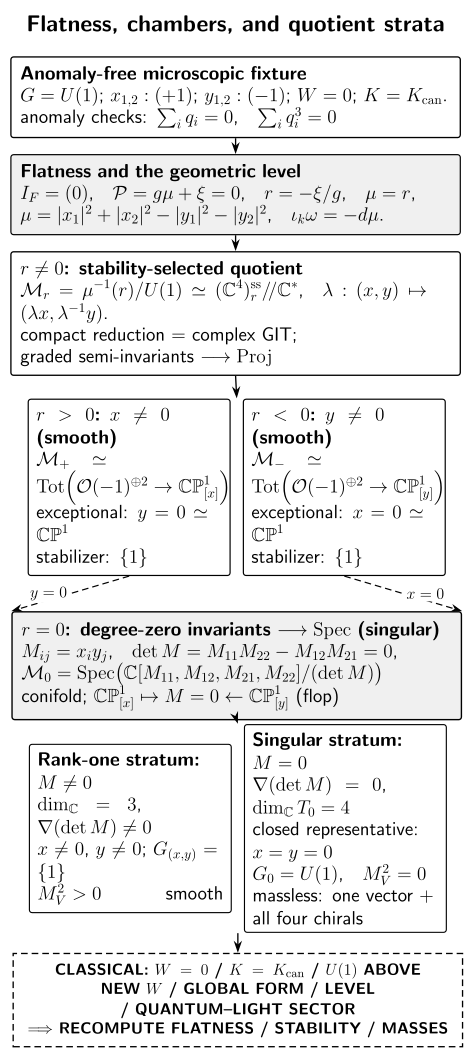
Exact classical quotient fixture for $G=U(1)$ with charges $(+1,+1,-1,-1)$, canonical $K$, and $W=0$. In the site convention $\mathcal P=g\mu+\xi$, D-flatness is $\mu=r$ with $r=-\xi/g$. The $r>0$ and $r<0$ stability choices give the two smooth small resolutions; degree-zero invariants at $r=0$ give $\det M=0$. The rank-one stratum has complex dimension three and trivial stabilizer, whereas at the origin the determinant Jacobian vanishes and the vector plus all four charged chirals are massless. The canonical derivation and primary-source locator accompany this fixture. The drawing is schematic and not to scale. Exact equations, adjacency, and independent checks (JSON).

Branch intersections

Consider a local vacuum equation $XY=0$. The solution is the union

$$\{X=0\}\cup\{Y=0\},$$

and the origin is singular because two branches meet. A low-energy expansion made on the $X=0$, $Y\neq0$ branch need not contain the degrees of freedom appropriate to the other branch. At the intersection, fields that were massive due to $Y\neq0$ can become light.

The correct procedure is:

1. decompose the vacuum ideal into branches;
2. determine the generic massless multiplets on each branch;
3. recompute the full quadratic action at the intersection;
4. include every newly massless multiplet before taking the infrared limit.

Counting tangent directions at the intersection often overcounts propagating moduli because some infinitesimal directions are obstructed at higher order. The full potential, not only its linearization, decides which directions extend to actual vacua.

Metric singularities from thresholds

Suppose a charged state has central-charge mass $M_\gamma(u)=|Z_\gamma(u)|$. In a local electric–magnetic frame in which $\gamma$ is electric, integrating out that state can give the holomorphic Abelian gauge coupling—equivalently, a second derivative of the prepotential—a logarithmic one-loop threshold in the vanishing special coordinate $a_\gamma=Z_\gamma$. Its coefficient and sign depend on the charge and on the convention for $\tau$. When $Z_\gamma(u_*)=0$, the coupling written without that state becomes singular. The singularity is physically valuable: monodromy around $u_*$ records the state’s charge. But the EFT used to derive the logarithm is invalid at $u_*$.

In Seiberg–Witten theory, an electric coordinate can make a monopole point look strongly coupled. Passing to a magnetic duality frame and including the light monopole hypermultiplet yields a weakly coupled local description Seiberg and Witten 1994, § 5.4, Eqs. (5.7)–(5.12), and § 5.6, Eq. (5.17), arXiv:hep-th/9407087. At more exceptional loci, mutually nonlocal charges can vanish simultaneously; no single electric–magnetic frame makes them all elementary, and the infrared limit can be an interacting Argyres–Douglas theory Argyres and Douglas 1995, Introduction, Eq. (1.1) and p. 2, § 4, Eq. (4.2), pp. 18–20, and § 5, pp. 29–31, arXiv:hep-th/9505062. The diagnostic distinction is charge pairing: if two vanishing charges have nonzero Dirac pairing, they cannot both be described as ordinary local electric fields in one frame.

Here those theories serve only as examples of the diagnostic. The global Seiberg–Witten analysis belongs to Singularities, Monodromies, and Global Geometry, while mutually nonlocal massless sectors and their fixed-point data belong to Argyres–Douglas Theories, Class S, and Interfaces.

A decision tree for the low-energy description

At a suspect point $p$:

1. Check the presentation. Does another coordinate chart remove the divergence? If yes, use the regular chart.
2. Check the variety. Does the Jacobian rank drop, or do irreducible branches meet? Record the local tangent cone and branch data.
3. Check gauge symmetry. Compute the stabilizer and vector mass matrix. Add any restored gauge multiplets.
4. Check matter and BPS masses. Diagonalize the full quadratic action. For each independently established BPS state, evaluate $M_\gamma=|Z_\gamma|$; $Z_\gamma(p)=0$ is necessary for that existing state to become massless, not evidence that every such lattice vector is populated. Add only light states whose existence or protected index is independently known. Mutual locality decides whether they admit one local duality frame, not whether they exist.
5. Check locality. If simultaneously light charges are mutually nonlocal, do not invent a local Lagrangian containing all of them. Look for an interacting fixed-point description and match its protected data.
6. Check control. State the energy window, distance from the singular locus, and corrections omitted.

The output should name both the new variables and the evidence for them. “Emergent” is a conclusion from spectra and scaling, not a synonym for “the metric diverges.”

Common pitfalls

Assuming every singularity is pathological. Moduli-space singularities often mark perfectly consistent points where an economical EFT changes variables or gains light fields.

Adding fields without checking charges. A vanishing mass suggests a state, but a local action requires mutually local electric charges in the chosen frame. Nonzero Dirac pairing is an obstruction.

Using only the Hessian of invariant coordinates. Gauge invariants can hide a massless vector multiplet. Always return to a representative microscopic configuration and compute its stabilizer.

Exercises

Let $u=xy$ describe the affine quotient of two fields with charges $+1$ and $-1$ at zero FI parameter.

1. Is the invariant variety singular at $u=0$?
2. What is the stabilizer of a nonzero representative and of the origin?
3. What does this example show about using algebraic smoothness as the only physical diagnostic?

Solution

The quotient is the complex line $\mathbb C_u$, so it is algebraically smooth even at $u=0$. For $u\neq0$, both $x$ and $y$ are nonzero and the $U(1)$ stabilizer is trivial. The closed representative of $u=0$ is $x=y=0$, whose stabilizer is all of $U(1)$. With $W=0$, the vector multiplet and both charged chiral multiplets are massless there: the vector mass, gauge-Yukawa mass, and chiral Hessian all vanish. Thus a smooth invariant variety can still contain a locus where the sigma-model field content is incomplete. Stabilizer and full quadratic-spectrum tests contain physical information not visible in the reduced coordinate ring.

References

• Argyres, Philip C., and Michael R. Douglas. “New Phenomena in $SU(3)$ Supersymmetric Gauge Theory.” Nuclear Physics B 448 (1995): 93–126. arXiv:hep-th/9505062.
• Luty, Markus A., and Washington Taylor IV. “Varieties of Vacua in Classical Supersymmetric Gauge Theories.” Physical Review D 53 (1996): 3399–3405. arXiv:hep-th/9506098.
• Seiberg, Nathan, and Edward Witten. “Electric–Magnetic Duality, Monopole Condensation, and Confinement in $\mathcal N=2$ Supersymmetric Yang–Mills Theory.” Nuclear Physics B 426 (1994): 19–52; erratum 430 (1994): 485–486. arXiv:hep-th/9407087.