Exact-Observable Identities as Duality Tests

An identity between exact observables is useful duality evidence only after both formulas describe the same background experiment. The comparison must translate parameters, global sectors, contact terms, decoupled factors, contours, and any defect labels. An independently proved integral identity can then establish equality of the defined protected observables and test a detailed duality dictionary, but it does not by itself establish equality of unprotected correlators or generic OPE data.

Required background. Use the hierarchy of duality checks and failure modes and the complete sphere matrix-model specification.

Helpful background. Holomorphic-block factorization explains identities that hold only after summing vacuum blocks or applying Stokes transformations.

The comparison record

Suppose theories $A$ and $B$ are proposed to be dual. A comparison has the form

$$Z_A[\mathcal B_A,D_A;\lambda_A] =e^{P_{\mathrm{local}}[\mathcal B_B;\lambda_B]} \mathcal N_{AB} Z_B[\mathcal B_B,D_B;\lambda_B], \qquad \lambda_B=f(\lambda_A).$$

Here $\mathcal B$ includes the manifold, spin or generalized spin structure, background bundles, preserved supercharge, and chamber; $D$ denotes any defect data; and $\lambda$ collects continuous and discrete parameters. The local exponential may encode background Chern–Simons terms or anomaly prefactors and is removable only to the extent allowed counterterms can shift it. The separate factor $\mathcal N_{AB}$ records declared changes of definition or normalization, such as a decoupled sector, gauge-volume factor, or a consistently included supersymmetric Casimir prefactor; it is not automatically local or scheme-removable. For compact Abelian background symmetries in three dimensions, for example, integer Chern–Simons shifts are scheme choices on spin manifolds while the fractional level is physical Closset et al. 2012, §§1–2. The counterterm analysis owns the general distinction.

A valid comparison matches:

• the manifold, orientation, spin structure, preserved supercharge, and background bundles;
• global gauge and flavor groups, including discrete quotients and one-form backgrounds;
• masses, FI terms, marginal couplings, theta angles, R charges, and fugacities;
• bundles, fluxes, instanton numbers, twisted sectors, and any discrete theta weights;
• the contour, residue or Stokes chamber, and analytic-continuation path;
• defect support, orientation, polarization, framing, and representation or magnetic label;
• decoupled free fields, Abelian factors, contact terms, and normalization.

Only after this translation should one record two separate labels. The validation mode is an analytic function identity, a formal-series identity, a precision-bounded numerical match, or a conditional calculation. The evidentiary reach is a protected-sector match or broader duality evidence. A theorem can establish the first validation mode, but “theorem” does not by itself say how much of either QFT has been compared.

The map below keeps three common exact constructions separate until a comparison record has made their inputs and qualifications commensurate. Read from the top into one branch at a time; the converging arrows indicate a shared comparison protocol, not equality among a sphere partition function, an index, and an instanton series.

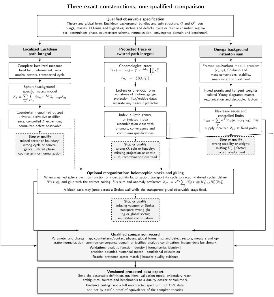
Three distinct exact constructions begin only after the theory, global data, supersymmetric background, sectors, cycles or regulators, counterterm class, normalization, convergence domain, and benchmark have been fixed. Localized integrals and protected traces may additionally admit vacuum-block decompositions with observable-specific gluings; dotted arrows mark that optional reorganization. An Omega-background instanton sum starts from a framed equivariant moduli problem, although on backgrounds such as $S^4$ its pole contributions can furnish the $Z_{\mathrm{np}}$ factor inside the localized branch. Every branch also has a direct route into the comparison record, whose strongest export is protected data with a stated validation mode and evidentiary reach—not an automatic proof of full QFT equivalence. Dashed arrows mark invalid definitions, missing sectors, uncontrolled analytic continuations or limits, and evidence overclaims. The map is schematic and not to scale; a structured semantic record preserves its complete labels and relationships.

Reflowing text equivalent

Qualified input. Fix the local Lagrangian or other theory definition together with the global gauge and flavor groups, discrete quotients, matter representations, couplings, anomalies, and regulator. Then fix the manifold, orientation, spin or generalized spin structure, background bundles, preserved supercharge, topological sector, and any defect. Record the physical or relative cycle, counterterm lattice, normalization choices, convergence domain, and at least one independent benchmark. Changing one of these entries can define a different background experiment even when the local formulas look similar.

Localized Euclidean path integral. Determine the full BPS locus, including disconnected flux and instanton sectors, and reduce the functional integral to the induced zero-mode measure, residual Weyl quotient, classical action, one-loop determinant, nonperturbative factors, and inherited integration cycle. The result is background-specific: examples include an $S^3$ Cartan integral, an $S^4$ Coulomb integral with pole instantons, and an $S^2$ flux sum. Before exporting a finite part, derivative, or phase, either quotient by allowed local supersymmetric counterterms or retain the fixed scheme, with normalization changes listed separately. Missing sectors or poles, field-space boundary terms, nonconvergence, an unfixed determinant phase or level lattice, and conflating counterterms with normalization all stop this branch.

Protected trace or twisted path integral. Choose $Q$, form $\Delta_Q=\tfrac12\{Q,Q^\dagger\}$, and admit only fugacities for charges commuting with $Q$ and $Q^\dagger$. Specify the trace domain, spin structure, gauge projection, global sectors, and convergence region before pairing noncohomological states. A Lagrangian evaluation may proceed through letters or one-loop determinants together with holonomy integrals, flux sums, and residue prescriptions. A path-integral realization can carry a supersymmetric Casimir prefactor outside the vacuum-normalized trace, so the two normalizations must not be silently identified Assel et al. 2015, eqs. (1.1)–(1.2) and §4. The outputs include superconformal indices, twisted indices, and elliptic genera, but they determine protected recombination classes rather than a unique short-multiplet spectrum. A noncommuting fugacity, continuum contribution, wrong spin structure, incomplete projection, omitted sector, divergent trace, or spectrum overclaim invalidates the stated conclusion.

Omega-background instanton sum. Begin with the framed instanton or ADHM moduli problem, its global gauge data, small-instanton compactification, stability chamber, and explicit $(\epsilon_1,\epsilon_2)$, Coulomb, mass, and counting-parameter conventions. Equivariant localization then replaces the resolved moduli integral by fixed points and their tangent and matter weights, producing a Nekrasov series with declared perturbative and decoupled factors. This technology is not disjoint from compact-background localization: on $S^4$, for example, north- and south-pole Omega-background functions provide the nonperturbative factors in the Coulomb integral. Prepotential and Nekrasov–Shatashvili limits require their own order of limits and asymptotic control. A wrong stability chamber or tangent character, a hidden physical-to-equivariant mass shift, a missing Abelian or center-of-mass factor, or an uncontrolled limit stops this branch.

Observable-specific blocks and gluing. A localized integral or protected trace may sometimes be reorganized into solid-torus blocks, but this is an additional conditional construction rather than a universal fourth definition. It requires isolated massive vacua or an explicitly enlarged spectral decomposition; a spanning set of relative cycles; paired $|q|<1$ and $|q|>1$ domains or a named resummation; and the correct gluing map, flux and discrete sectors, contact prefactor, and analytic-continuation path. A block basis can jump across a Stokes wall while the glued observable remains unchanged only if the partner basis and kernel undergo the contragredient transport. Colliding vacua, an unlifted continuum, an incomplete cycle basis, or a missing gluing sector changes or defeats the factorization claim.

Qualified comparison and export. Compare outputs only after matching the full theory dictionary; background and supercharge; global, flux, instanton, twisted, and defect sectors; continuous and discrete parameter maps; contours, chambers, and analytic-continuation paths; counterterms and normalizations; and convergence, truncation, numerical error, and benchmarks. Record the validation mode—analytic function identity, formal-series identity, precision-bounded numerical match, or conditional calculation—and separately record the evidentiary reach—protected-sector match or broader duality evidence. One may then export protected degeneracies or recombination classes, anomaly and contact data, effective couplings in controlled limits, and duality evidence within the tested sectors. Neither label, by itself, reconstructs generic OPE data or proves equivalence of the full quantum field theories.

A convention-complete Seiberg-index identity

Consider four-dimensional $\mathcal N=1$ $SU(N_c)$ SQCD with $N_c\geq2$ and $N_f\geq N_c+2$ flavors. Its magnetic description has

$$\widetilde N_c=N_f-N_c, \qquad r=R(Q)=R(\widetilde Q) =1-\frac{N_c}{N_f} =\frac{\widetilde N_c}{N_f}.$$

This is the anomaly-free R symmetry. It is the superconformal R symmetry in the interacting conformal window $3N_c/2<N_f<3N_c$; outside that window the same meromorphic integral identity should not be mislabeled as an interacting-SCFT statement. Seiberg gives the magnetic rank, charges, mesons, baryons, and superpotential in Seiberg 1995, §§1–3.

For $|p|,|q|<1$, define the elliptic Gamma function

$$\Gamma_e(z;p,q) =\prod_{j,k\geq0} \frac{1-p^{j+1}q^{k+1}z^{-1}} {1-p^jq^kz}.$$

Choose flavor fugacities $y_i,\widetilde y_i$ with $\prod_i y_i=\prod_i\widetilde y_i=1$ and baryon fugacity $v$, and set

$$s_i=(pq)^{r/2}v y_i, \qquad t_i=(pq)^{r/2}v^{-1}\widetilde y_i^{-1}.$$

Then

$$\prod_{i=1}^{N_f}s_it_i =(pq)^{N_fr} =(pq)^{\widetilde N_c}.$$

Thus the balancing condition is the anomaly-free R-charge constraint together with the special-unitary flavor constraints. Below, $(p;p)_\infty=\prod_{j\geq1}(1-p^j)$, and similarly for $q$.

It is useful to define one integral family. For $n\geq2$, let

$$\mathcal J_n(s,t) ={\frac{(p;p)_\infty^{n-1}(q;q)_\infty^{n-1}}{n!}} \oint \prod_{a=1}^{n-1}\frac{dz_a}{2\pi i z_a} \,\mathcal Z_n(z;s,t), \qquad z_n=\left(\prod_{a=1}^{n-1}z_a\right)^{-1},$$

where

$$\mathcal Z_n(z;s,t) =\frac{ \displaystyle\prod_{a=1}^{n}\prod_{i=1}^{N_f} \Gamma_e(s_i z_a;p,q)\Gamma_e(t_i z_a^{-1};p,q)} {\displaystyle\prod_{\substack{1\leq a,b\leq n\\a\ne b}} \Gamma_e(z_a/z_b;p,q)}.$$

Initially the contours are unit circles separating the pole sequences that approach zero from those that approach infinity. Define $S=\prod_i s_i$ and $T=\prod_i t_i$. Rains’s $A_{N_c-1}\leftrightarrow A_{\widetilde N_c-1}$ transformation then gives

$$\mathcal J_{N_c}(s,t) =\prod_{i,j=1}^{N_f}\Gamma_e(s_it_j;p,q)\, \mathcal J_{\widetilde N_c} \left(S^{1/\widetilde N_c}s^{-1}, T^{1/\widetilde N_c}t^{-1}\right).$$

The notation $S^{1/\widetilde N_c}s^{-1}$ means the list whose $i$th entry is $S^{1/\widetilde N_c}s_i^{-1}$. In the initial domain one may take the individual matter arguments inside the unit circle; Rains’s theorem then supplies a meromorphic continuation to generic balanced parameters, with contour deformations and crossed residues treated explicitly Rains 2010, Theorem 4.1.

The transformed arguments make the magnetic map visible:

$$\begin{aligned} S^{1/\widetilde N_c}s_i^{-1} &=(pq)^{(1-r)/2} v^{N_c/\widetilde N_c}y_i^{-1},\\ T^{1/\widetilde N_c}t_i^{-1} &=(pq)^{(1-r)/2} v^{-N_c/\widetilde N_c}\widetilde y_i. \end{aligned}$$

Therefore the magnetic quarks have R charge $1-r=N_c/N_f$ and baryon charges $\pm N_c/\widetilde N_c$. The $N_f^2$ factors outside the magnetic integral are the elementary mesons

$$M^i{}_j=Q^i\widetilde Q_j, \qquad s_it_j=(pq)^r y_i\widetilde y_j^{-1},$$

so $R(M)=2r$. The magnetic superpotential $W=Mq\widetilde q$ then has R charge $2r+2(1-r)=2$. Choosing the roots of $S$ and $T$ amounts to choosing a baryon-fugacity branch; gauge-invariant magnetic operators are single-valued after the global quotient is fixed. Dolan and Osborn identify this exact transformation with the electric and magnetic superconformal indices in Dolan and Osborn 2009, §6, especially eqs. (6.9)–(6.13).

What this test establishes

The two integrals are derived from different ultraviolet gauge theories, while the equality is proved by a special-function theorem that does not assume the physical duality. It simultaneously checks:

• the magnetic rank $N_f-N_c$;
• meson multiplicities and charges;
• the nonanomalous R-symmetry and flavor representations;
• baryon-charge matching;
• the magnetic-quark R and baryon charges;
• the balancing condition and infinitely many protected-state coefficients.

This is stronger than matching a few series coefficients, but it remains an identity of the defined supersymmetric indices. Long multiplets cancel, generic OPE coefficients are absent, and the ordinary integral does not distinguish every possible global form or line-operator lattice. Those require refinements by the corresponding background sectors.

Instanton and defect refinements

An instanton comparison has the schematic form

$$Z_{\rm inst}^A(q_A,a_A,m_A;\epsilon_A) =Z_{\rm dec}\,e^{P_{\rm local}} Z_{\rm inst}^B(q_B,a_B,m_B;\epsilon_B).$$

The Omega-background convention card must be translated before coefficients are compared: $U(N)$ versus $SU(N)$ factors, the phase of $q$, physical versus equivariant masses, and the small-instanton compactification can all create a false mismatch. Agreement through instanton number $K$ establishes only a coefficient match through $q^K$ unless an independent recursion or analytic theorem upgrades it.

A supersymmetric defect inserts an operator or modifies boundary conditions in the localized integral. A duality claim must then map both its support and label:

$$Z_A[D_A] \stackrel{?}{=} e^{P_{\mathrm{local}}} Z_B[D_B].$$

In block or index realizations, Wilson, vortex, and ‘t Hooft defects can act by multiplication or difference operators. If $\mathcal U$ is the duality kernel between the two chosen polarizations, the stronger test is the intertwining relation

$$\mathcal U\,\widehat D_A =\widehat D_B\,\mathcal U$$

on a specified function space and contour. This tests the operator map more strongly than the vacuum partition function alone. Fusion and linked-defect observables add further independent constraints only when support, orientation, framing, global charges, and contact terms are matched.

Independence and evidence ceiling

Comparison	Strongest immediate conclusion	Still missing
Numerical samples with certified truncation and rounding errors	Equality at the sampled parameters within the reported bound	A statement between sample points
Series agreement through order $K$	Protected coefficients agree through order $K$	Higher orders and nonperturbative completion
Identity derived using the proposed duality	Internal consistency of that derivation	Logical independence
Independent special-function theorem	Exact equality of the fully defined protected observables	Unprotected data and omitted global refinements
Identity plus mapped defects and global sectors	Strong protected-sector and extended-operator evidence	A proof of the full QFT equivalence

None of these steps alone proves equality of all unprotected observables. Conversely, a mismatch is not immediately a disproof: first test counterterm phases, fugacity maps, missing sectors, decoupled factors, and contour chambers. A mismatch that survives those checks is genuine evidence against the proposed dictionary or its stated domain.

A comparison protocol

1. Freeze both complete theory specifications, global forms, backgrounds, and the proposed parameter map.
2. Derive both exact-observable formulas independently in one normalization, recording shared inputs.
3. Translate every continuous and discrete parameter and verify that the map is invertible on the claimed domain.
4. Separate allowed local factors, preserving fractional anomaly and contact data.
5. Match flux, instanton, twisted, and defect sectors before summing them.
6. Establish one common convergence domain and record every contour deformation used for analytic continuation.
7. Check a free limit, a low-order coefficient, or another benchmark that can fail independently.
8. Prove the identity, or report the sampling points, precision, truncation error, and conditioning of a numerical test.
9. Repeat with a background or defect that tests a genuinely new part of the dictionary.
10. State the strongest bounded conclusion and list the untested sectors.

Failure modes

A tautological match. If one formula was obtained from the other by assuming the proposed duality, equality is a consistency check, not independent evidence.

A missing global sector. Integrals over the same Lie algebra can represent different global gauge groups. Discrete bundles, one-form backgrounds, and line lattices must be compared separately.

A contact-term mismatch. An integer scheme shift may be harmless while a fractional background Chern–Simons mismatch is physical. Calling the entire phase “a convention” can erase an anomaly test.

A wrong fugacity root. Fractional baryon charges in the magnetic description require a compatible global quotient. A branch chosen separately for each gauge-variant field can spoil gauge-invariant baryons.

Untracked analytic continuation. A theorem in one pole-separation domain extends meromorphically only with the contour deformed and crossed residues included.

A hidden decoupled factor. Free singlets, center-of-mass multiplets, and Abelian instanton factors can multiply only one side unless explicitly removed or matched.

Unbounded numerics. Decimal agreement without truncation, quadrature, and floating-point error bounds is a plot-level observation, not a precision statement.

Evidence inflation. Equality of a protected trace does not reconstruct generic OPE coefficients or prove full equivalence of the two quantum field theories.

Exercises

1. Reconstruct the magnetic charge map

Starting from $s_i=(pq)^{r/2}vy_i$, derive the R charge and baryon charge of the magnetic quark argument $S^{1/\widetilde N_c}s_i^{-1}$.

Solution

Since $S=(pq)^{N_fr/2}v^{N_f}$,

$$S^{1/\widetilde N_c}s_i^{-1} =(pq)^{\frac{N_fr}{2\widetilde N_c}-\frac r2} v^{\frac{N_f}{\widetilde N_c}-1}y_i^{-1}.$$

Using $r=\widetilde N_c/N_f$ and $N_f-\widetilde N_c=N_c$, the exponents become

$$\frac{N_fr}{\widetilde N_c}-r=1-r, \qquad \frac{N_f}{\widetilde N_c}-1 =\frac{N_c}{\widetilde N_c}.$$

Because an index argument carries $(pq)^{R/2}$, the magnetic quark has $R=1-r$ and baryon charge $N_c/\widetilde N_c$.

2. Explain the meson factor

Why does the index identity contain $\prod_{i,j}\Gamma_e(s_it_j;p,q)$ outside the magnetic gauge integral?

Solution

The electric meson $M^i{}_j=Q^i\widetilde Q_j$ has elliptic-Gamma argument $s_it_j$. In the magnetic description it is an elementary gauge singlet, so all $N_f^2$ components contribute

$$\prod_{i,j=1}^{N_f}\Gamma_e(s_it_j;p,q).$$

Removing this factor would erase the meson operators and spoil their flavor and R-charge matching.

3. Classify a finite-order match

Two instanton series agree through $q^4$ after a parameter map, but no recursion or analytic identity is known. What has been established?

Solution

Only the protected coefficients through instanton number four have been matched, in the stated convention and parameter domain. The result is useful evidence and can expose rank, mass-shift, or decoupled-factor errors, but it says nothing by itself about $q^5$ and higher terms, convergence of the all-instanton sum, or unprotected observables.

References

• Assel, B., D. Cassani, L. Di Pietro, Z. Komargodski, J. Lorenzen, and D. Martelli. “The Casimir Energy in Curved Space and Its Supersymmetric Counterpart.” Journal of High Energy Physics 2015, no. 7 (2015): 043. DOI; Open PDF.
• Closset, C., T. T. Dumitrescu, G. Festuccia, Z. Komargodski, and N. Seiberg. “Comments on Chern–Simons Contact Terms in Three Dimensions.” Journal of High Energy Physics 2012, no. 9 (2012): 091. DOI; Open PDF.
• Dolan, F. A., and H. Osborn. “Applications of the Superconformal Index for Protected Operators and $q$-Hypergeometric Identities to $N=1$ Dual Theories.” Nuclear Physics B 818 (2009): 137–178. DOI; Open PDF.
• Rains, E. M. “Transformations of Elliptic Hypergeometric Integrals.” Annals of Mathematics 171 (2010): 169–243. DOI; Open PDF.
• Seiberg, N. “Electric–Magnetic Duality in Supersymmetric Non-Abelian Gauge Theories.” Nuclear Physics B 435 (1995): 129–146. DOI; Open PDF.