Q-Cohomology, Hodge Decomposition, and Zero-Energy States

$Q$-cohomology and zero-energy states agree when the supercharge is a genuine closed differential, its adjoint and Hamiltonian use compatible domains, and the relevant Hodge decomposition holds. In finite dimension these facts are automatic once an inner product is chosen. For an infinite-dimensional Hilbert complex, harmonic states always represent reduced cohomology; ordinary cohomology has unique harmonic representatives only when the image of $Q$ is closed. Compact elliptic de Rham quantum mechanics satisfies these hypotheses, while noncompact spaces and boundaries require additional analysis.

Required background. Supercharges and partner Hamiltonians fixes the operator normalization. Chains, homology, cohomology, and exact sequences supplies quotient cohomology, and de Rham cohomology supplies the geometric complex. Helpful background. Differential forms, integration, orientation, and Stokes’ theorem clarifies the adjoint and boundary terms.

A supercharge is a differential

Let $\mathcal H=\bigoplus_k\mathcal H^k$ be a finite-dimensional graded complex Hilbert space and let

$$Q:\mathcal H^k\longrightarrow\mathcal H^{k+1}, \qquad Q^2=0.$$

The degree-$k$ cohomology is

$$H_Q^k=\frac{\ker(Q:\mathcal H^k\to\mathcal H^{k+1})} {\operatorname{im}(Q:\mathcal H^{k-1}\to\mathcal H^k)}.$$

A $Q$-closed vector represents a class; adding a $Q$-exact vector does not change it. This quotient is algebraic and does not yet select a preferred state. The inner product supplies $Q^\dagger$ and the $Q$-Laplacian

$$\Delta_Q=QQ^\dagger+Q^\dagger Q=2H.$$

A vector is harmonic when $\Delta_Q\psi=0$. Positivity yields the decisive equivalence

$$\langle\psi|\Delta_Q|\psi\rangle =\lVert Q\psi\rVert^2+\lVert Q^\dagger\psi\rVert^2,$$

so

$$\ker\Delta_Q=\ker Q\cap\ker Q^\dagger=\ker H.$$

Thus “harmonic” and “zero energy” are the same Hilbert-space condition. The remaining question is whether harmonic vectors represent cohomology completely and uniquely.

Finite-dimensional Hodge decomposition

Nilpotence makes $\operatorname{im}Q$ orthogonal to $\operatorname{im}Q^\dagger$. The orthogonal complement of their sum consists exactly of vectors annihilated by both $Q$ and $Q^\dagger$. Therefore

$$\mathcal H =\operatorname{im}Q \oplus\operatorname{im}Q^\dagger \oplus\ker\Delta_Q.$$

This is the finite Hodge decomposition. It implies the harmonic-representative theorem. If $Q\psi=0$, decompose

$$\psi=Q\alpha+Q^\dagger\beta+h, \qquad h\in\ker\Delta_Q.$$

Applying $Q$ gives $QQ^\dagger\beta=0$, hence

$$\lVert Q^\dagger\beta\rVert^2 =\langle\beta|QQ^\dagger|\beta\rangle=0.$$

So $\psi=Q\alpha+h$: every class has a harmonic representative. If a harmonic $h$ is also exact, $h=Q\alpha$, then

$$\lVert h\rVert^2=\langle h|Q\alpha\rangle =\langle Q^\dagger h|\alpha\rangle=0,$$

so that representative is unique. Degree by degree,

$$H_Q^k\cong\ker(\Delta_Q|_{\mathcal H^k}).$$

An exact matrix fixture

Consider the two-term complex $0\to\mathbb C^2\xrightarrow{A}\mathbb C^3\to0$ with standard inner products and

$$A= \begin{pmatrix} 1&0\\ 0&0\\ 0&0 \end{pmatrix}.$$

The complete correspondence is visible without diagonalization:

Quantity	Even degree $\mathbb C^2$	Odd degree $\mathbb C^3$
Hamiltonian	$H_{\bar0}=\tfrac12\operatorname{diag}(1,0)$	$H_{\bar1}=\tfrac12\operatorname{diag}(1,0,0)$
Positive-energy subspace	$\operatorname{span}\{e_1\}$	$\operatorname{span}\{f_1\}$
Harmonic subspace	$\operatorname{span}\{e_2\}$	$\operatorname{span}\{f_2,f_3\}$
Cohomology dimension	$\dim H_Q^0=1$	$\dim H_Q^1=2$

$A$ pairs $e_1$ with $f_1$ at energy $1/2$. The three unpaired harmonic vectors are precisely the three cohomology representatives, and the signed zero-mode count is $1-2=-1$. This finite fixture also shows that cohomology is more informative than the single integer index.

Cohomology–Hodge correspondence

The figure organizes the same exact matrix fixture by following each subspace. Inspect the positive-energy arrow $e_1\leftrightarrow f_1$, then compare the kernel modulo the image with the unpaired harmonic representatives.

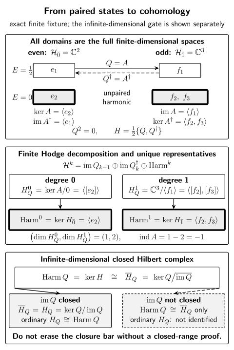
Exact finite-dimensional correspondence for $0\to\mathbb C^2\xrightarrow{A}\mathbb C^3\to0$ with $Ae_1=f_1$ and $Ae_2=0$. The pair $e_1\leftrightarrow f_1$ has energy $1/2$; $e_2$, $f_2$, and $f_3$ are simultaneously harmonic, unpaired, and representatives of $Q$-cohomology. In an infinite-dimensional complex the same diagram represents reduced cohomology unless the relevant image is closed.

The semantic table makes every node and arrow explicit:

Exact object	Even degree $\mathbb C^2$	Odd degree $\mathbb C^3$	Consequence
$\ker Q$	$\operatorname{span}\{e_2\}$	$\operatorname{span}\{f_1,f_2,f_3\}$	These are the closed vectors before quotienting.
$\operatorname{im}Q$	$0$	$\operatorname{span}\{f_1\}$	The odd vector $f_1$ is exact.
$\operatorname{im}Q^\dagger$	$\operatorname{span}\{e_1\}$	$0$	The adjoint sends $f_1$ back to $e_1$.
$\ker Q\cap\ker Q^\dagger$	$\operatorname{span}\{e_2\}$	$\operatorname{span}\{f_2,f_3\}$	These are the harmonic, zero-energy subspaces.
Quotient representatives	$[e_2]$	$[f_2]$, $[f_3]$	They form bases of $H_Q^0$ and $H_Q^1$.
Positive-energy action	$Qe_1=f_1$	$Q^\dagger f_1=e_1$	$e_1\leftrightarrow f_1$ is the paired level at $E=1/2$.

Finite dimensionality makes every image closed. For a Hilbert complex the table remains valid with $\operatorname{im}Q$ and $\operatorname{im}Q^\dagger$ replaced by their closures; identifying the displayed quotient with ordinary rather than reduced cohomology requires the closed-range hypothesis developed next.

Infinite-dimensional Hilbert complexes

For an unbounded $Q$, the equation $Q^2=0$ must mean

$$Q(\operatorname{Dom}Q)\subset\operatorname{Dom}Q, \qquad Q(Q\psi)=0 \quad\text{for every }\psi\in\operatorname{Dom}Q.$$

Assume $Q$ is densely defined and closed. Then the weak orthogonal decomposition uses closures,

$$\mathcal H =\overline{\operatorname{im}Q} \oplus\overline{\operatorname{im}Q^\dagger} \oplus\ker\Delta_Q,$$

with the Laplacian defined on the intersection of the appropriate composite domains. Harmonic vectors naturally identify with the reduced cohomology

$$\overline H_Q =\frac{\ker Q}{\overline{\operatorname{im}Q}}.$$

If $\operatorname{im}Q$ is closed, reduced and ordinary cohomology agree and the strong Hodge decomposition follows. If it is not closed, $\ker Q/\operatorname{im}Q$ can be non-Hausdorff: exact vectors can converge to a non-exact vector. A harmonic state then classifies the reduced class, not necessarily the algebraic quotient. This is the central analytic qualification in the Hilbert-complex framework Brüning and Lesch 1992, §§1–2, pp. 88–103.

Compactness is a sufficient mechanism in the geometric example below, not a universal requirement. More generally one may establish closed range by a spectral gap above zero, a Poincaré estimate on the orthogonal complement of the kernel, or Fredholmness.

De Rham supersymmetric quantum mechanics

Let $M$ be a smooth, compact, oriented Riemannian manifold without boundary. Take

$$\mathcal H=L^2\Omega^\bullet(M;\mathbb C), \qquad Q=d, \qquad Q^\dagger=\delta.$$

Form degree is fermion number, so even and odd forms give the two $\mathbb Z_2$ sectors. The Hamiltonian is half the Hodge Laplacian,

$$H=\frac12(d\delta+\delta d)=\frac12\Delta_{\mathrm{dR}}.$$

Ellipticity and compactness give a self-adjoint operator with compact resolvent, finite-dimensional kernel, and closed range. The analytic Hodge theorem therefore identifies

$$H^k_{\mathrm{dR}}(M;\mathbb C) \cong\mathcal H^k_{\mathrm{harm}}(M) \cong\{\text{supersymmetric ground states of fermion number }k\}.$$

With the normalization used here, the two Hermitian supercharges are $(d+\delta)/\sqrt2$ and $i(d-\delta)/\sqrt2$; each squares to $H=\Delta_{\mathrm{dR}}/2$. Witten uses the unscaled pair, for which the Hamiltonian is the full form Laplacian Witten 1982, §2, pp. 665–666. Supersymmetric path-integral formulations connect the corresponding graded trace to the index of an elliptic complex Alvarez-Gaumé 1983, pp. 161–173, but the operator statement above does not rely on a formal path integral.

Motion on a circle

For a circle of radius $R$, use $\theta\sim\theta+2\pi$ and metric $\mathrm ds^2=R^2\mathrm d\theta^2$. Fourier modes give

$$d(e^{in\theta})=in e^{in\theta}\mathrm d\theta, \qquad \Delta_{\mathrm{dR}}e^{in\theta} =\frac{n^2}{R^2}e^{in\theta},$$

and the same eigenvalue on $e^{in\theta}\mathrm d\theta$. Therefore

$$E_n=\frac{n^2}{2R^2}.$$

For every $n\ne0$, $d$ and $\delta$ pair a zero-form mode with a one-form mode. At $n=0$ there are exactly two harmonic states: the constant function in degree zero and the constant one-form in degree one. Hence

$$\dim H^0(S^1)=1, \qquad \dim H^1(S^1)=1.$$

Supersymmetry is unbroken, although the signed even-minus-odd count vanishes. This is the canonical counterexample to the claim that zero Witten index proves breaking.

Boundaries and deformations

If $M$ has a boundary, integration by parts produces a boundary pairing. Absolute and relative elliptic boundary conditions lead to different complexes and respectively to ordinary and relative de Rham cohomology. Merely declaring the Laplacian self-adjoint does not ensure that $d$ maps the chosen domain into itself. The continuum and boundary page gives an interval example.

A family $Q_t=S_t^{-1}QS_t$ has isomorphic algebraic cohomology whenever $S_t$ is invertible and preserves the relevant domains. In a Hilbert space, preserving physical cohomology also requires control of $S_t$ and $S_t^{-1}$ in the topology used for normalizability. On a compact manifold, multiplication by $e^{tf}$ is bounded and invertible for every finite $t$. On a noncompact manifold it can be unbounded and can create or remove $L^2$ representatives. The Morse-deformation page makes this distinction explicit.

Common pitfalls

Closed is not harmonic. $Q\psi=0$ defines a cohomology representative. Harmonicity also requires $Q^\dagger\psi=0$ and depends on the inner product.

The quotient may need a closure. In infinite dimension, replacing $\operatorname{im}Q$ by its closure changes ordinary cohomology to reduced cohomology. The replacement is harmless only after closed range is proved.

Topology does not determine every wavefunction. Betti numbers count harmonic representatives on a compact manifold, but the representatives themselves depend on the metric. Their number is topological; their profiles are not.

Exercises

Uniqueness of the harmonic representative. Why can an exact harmonic vector not be nonzero?

Solution

If $h=Q\alpha$ and $Q^\dagger h=0$, then $\lVert h\rVert^2=\langle h|Q\alpha\rangle=\langle Q^\dagger h|\alpha\rangle=0$. Thus $h=0$. The step uses the adjoint relation on compatible domains; a purely formal integration by parts would not suffice on a space with boundary.

Normalized vacua on the circle. For the circle with $ds^2=R^2d\theta^2$, normalize the harmonic zero-form and harmonic one-form. What is their signed Witten index?

Solution

The volume form is $R\,d\theta$. A constant zero-form therefore has unit norm when

$$\phi_0=\frac{1}{\sqrt{2\pi R}}.$$

Since the pointwise norm of $d\theta$ is $1/R$, the normalized harmonic one-form is

$$\phi_1=\sqrt{\frac{R}{2\pi}}\,d\theta.$$

There is one even and one odd zero-energy state, so supersymmetry is unbroken but the signed index is $1-1=0$.

Why the closure changes cohomology. Let $A:\ell^2\to\ell^2$ be the bounded injective operator $(Ax)_n=x_n/n$, and form the two-term complex $0\to\ell^2\xrightarrow{A}\ell^2\to0$. Show that $\operatorname{im}A$ is dense but not closed. Compare ordinary odd cohomology, reduced odd cohomology, and odd harmonic vectors.

Solution

Every finite sequence lies in $\operatorname{im}A$, so the range is dense. It is not closed: the vector $y_n=1/n$ lies in $\ell^2$ but not in the range, because a preimage would have $x_n=1$, which is not square-summable. Its finite truncations do lie in the range and converge to $y$.

In odd degree, $\ker Q=\ell^2$. Thus the ordinary quotient $\ell^2/\operatorname{im}A$ is nonzero and non-Hausdorff, whereas

$$\overline H_Q^1 =\frac{\ell^2}{\overline{\operatorname{im}A}} =0.$$

Because $A^\dagger=A$ and $A$ is injective, the odd harmonic space $\ker A^\dagger$ is also zero. Harmonic vectors therefore reproduce reduced, not ordinary, cohomology in this nonclosed-range example.

References

• Alvarez-Gaumé, Luis. “Supersymmetry and the Atiyah–Singer Index Theorem.” Communications in Mathematical Physics 90, no. 2 (1983): 161–173. doi:10.1007/BF01205500.
• Brüning, Jochen, and Matthias Lesch. “Hilbert Complexes.” Journal of Functional Analysis 108, no. 1 (1992): 88–132. doi:10.1016/0022-1236(92)90147-B.
• Witten, Edward. “Supersymmetry and Morse Theory.” Journal of Differential Geometry 17, no. 4 (1982): 661–692. doi:10.4310/jdg/1214437492.