Pseudomoduli, Quantum Lifting, and Metastability

A pseudomodulus is a classically flat scalar direction whose vacuum energy is nonzero and whose heavy spectrum varies along the flat direction. Quantum fluctuations can then generate a potential without restoring supersymmetry. This page diagonalizes the full field-dependent spectrum of a canonical O’Raifeartaigh model, derives its Coleman–Weinberg curvature, and then draws a sharp line between a loop-stabilized local minimum and a metastable vacuum with a calculable decay rate.

Required background. The tree-level model, order parameter, and tachyon boundary are established on O’Raifeartaigh and Fayet–Iliopoulos Model Laboratories. The quantum potential is a 1PI object; use The 1PI Effective Action and Mean-Field Equations for its definition and scheme dependence.

Helpful background. A lifetime claim uses Bounce Solutions and False-Vacuum Boundary Conditions after the local spectrum has been checked.

A pseudomodulus with an exact field-dependent spectrum

Take canonical chiral multiplets and

$$W=fX+\frac h2X\phi_1^2+m\phi_1\phi_2, \qquad f,h,m>0.$$

Along

$$\phi_1=\phi_2=0, \qquad V_0=f^2,$$

the complex field $X$ is flat at tree level and $F_X=-f$. Define the dimensionless quantities

$$y=\frac{hf}{m^2}, \qquad z=\frac{h|X|}{m}.$$

We restrict first to $0<y<1$, the tachyon-free branch found from the spectrum at $X=0$. A phase rotation makes $hX$ real for purposes of diagonalizing the quadratic form.

The two heavy Weyl fermions have mass matrix

$$\mathcal M_F= \begin{pmatrix} hX&m\\ m&0 \end{pmatrix},$$

so the eigenvalues of $\mathcal M_F^\dagger\mathcal M_F$ are

$$m_{F,\pm}^2 =m^2\left[ 1+\frac{z^2}{2} \pm\frac z2\sqrt{z^2+4} \right].$$

After the phase of $X$ is fixed, the real and imaginary quadratic fluctuations form two $2\times2$ blocks,

$$\mathcal M_{B,s}^2 =m^2 \begin{pmatrix} 1+z^2+sy & z\\ z & 1 \end{pmatrix}, \qquad s=\pm1.$$

Their determinants are $m^4(1+sy)$. Diagonalizing the blocks gives the four real heavy-scalar masses

$$m_{B,s,\pm}^2 =m^2\left[ 1+\frac{z^2+sy}{2} \pm\frac12\sqrt{(z^2+sy)^2+4z^2} \right].$$

Three checks catch most normalization mistakes:

1. At $z=0$, the scalar set is $m^2\{1+y,1,1,1-y\}$ and the two fermion masses squared are both $m^2$.
2. For each $s$, the product of the two dimensionless scalar eigenvalues is $1+sy$; the smallest product is $1-y>0$.
3. The tree-level supertrace obeys $\operatorname{STr}\mathcal M^2=0$.

The second check proves that every heavy scalar eigenvalue is positive for all finite $z$ when $0<y<1$: each pair has positive sum and positive product. At $y=1$, one mode is massless; at $y>1$, a tachyon appears. A loop expansion about the nominal valley is not a controlled vacuum calculation on that side of the boundary.

The spectrum also reveals a large-$|X|$ subtlety. Because $\det\mathcal M_F=-m^2$, one fermion becomes heavy like $h|X|$ while the other becomes light like $m^2/(h|X|)$; the small member of each scalar pair becomes light as well. Fixed-order logarithms and a single-field Wilsonian description therefore require reorganization at sufficiently large $z$ even though no scalar is tachyonic.

Coleman–Weinberg lifting

In a mass-independent $\overline{\rm DR}$-type scheme, the one-loop contribution from the four real bosons and two Weyl fermions is

$$\begin{aligned} V_1(X)=\frac{1}{64\pi^2}\Bigg\{& \sum_{s=\pm1}\sum_{t=\pm1} m_{B,s,t}^4 \left(\log\frac{m_{B,s,t}^2}{\mu^2}-\frac32\right)\\ &-2\sum_{t=\pm1}m_{F,t}^4 \left(\log\frac{m_{F,t}^2}{\mu^2}-\frac32\right) \Bigg\}. \end{aligned}$$

This is the Coleman–Weinberg supertrace evaluated on a nonsupersymmetric background Coleman and Weinberg 1973, pp. 1888–1910. Field-independent contributions from the massless goldstino and tree-level pseudomodulus vanish in dimensional regularization. Counterterms fix the additive vacuum energy and parameters; derivatives at an extremum, expressed in renormalized quantities at a stated scale, carry the physical local information.

Expanding the exact spectrum near $X=0$ gives

$$V_{\rm eff}(X) =f^2+V_1(0)+m_X^2|X|^2+O(|X|^4),$$

with

$$m_X^2 =\frac{h^2m^2}{64\pi^2}\,C(y),$$

and

$$C(y)=\frac{2}{y}\left[ (1+y)^2\log(1+y) -(1-y)^2\log(1-y)-2y \right].$$

For $0<y<1$, $C(y)>0$, so the positive one-loop curvature locally stabilizes the pseudomodulus at the R-symmetric point $X=0$ Shih 2008, Appendix A.1, pp. 13–14. In the weak-splitting limit,

$$C(y)=\frac43y^2+\frac{2}{15}y^4+O(y^6),$$

and therefore

$$m_X^2=\frac{h^4f^2}{48\pi^2m^2} +O\!\left(\frac{h^6f^4}{m^6}\right).$$

This provides a quantitative cross-check: the curvature vanishes quadratically with the supersymmetry-breaking splitting $y$ and is one-loop suppressed.

The figure below places three often-confused statements in one comparison: the exact tree-level stability of the nominal O’Raifeartaigh valley; the additional validity gate derived in Nonlinear Goldstino Dynamics and Constrained Effective Theory; and the distinct zero-soft and large-soft paths of the two-chiral benchmark derived in Soft Breaking, Spurions, and Controlled Decoupling, where $r=m_s^2/|m|^2$ and $\beta=|b|/|m|^2$.

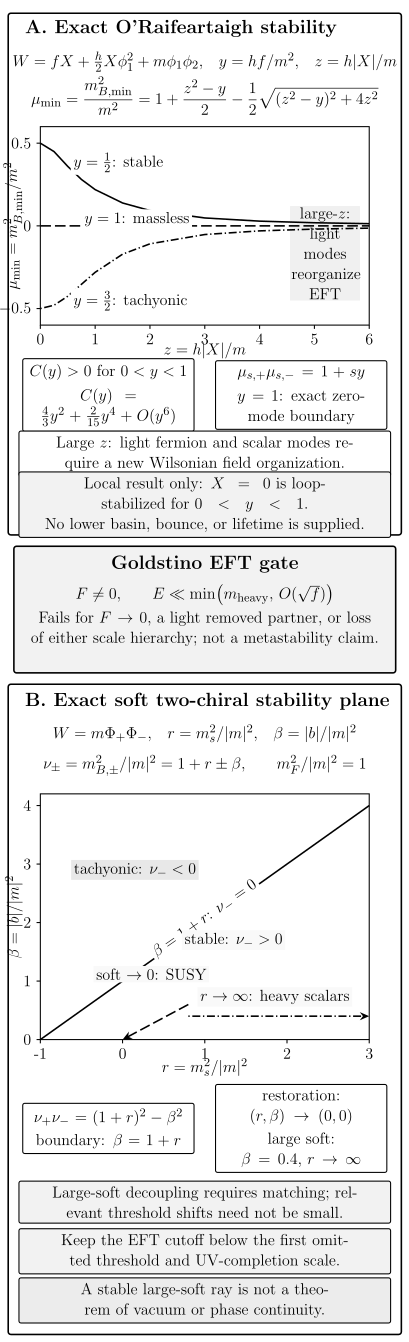
Exact data for the displayed benchmark models. Panel A shows the minimum tree-level O’Raifeartaigh scalar eigenvalue and the positive one-loop curvature only on the controlled $0<y<1$ branch; it supplies neither a lower basin nor a lifetime. The middle gate adds $F\neq0$ and $E\ll\min(m_{\rm heavy},\Lambda_{\rm NL})$. Panel B gives the exact boundary $\beta=1+r$ for the two-chiral soft benchmark: the zero-soft origin restores its supersymmetric spectrum, whereas the large-$r$ ray requires matching and proves no phase-continuity theorem. Structured figure data.

Pseudomodulus stability, nonlinear-EFT gate, and soft decoupling — print equivalent

This reflow preserves the figure’s quantitative curves, validity gate, and limiting statements at readable print size.

Panel A: exact O’Raifeartaigh stability

With y = hf/m² and z = h|X|/m, the smallest normalized scalar eigenvalue is μ_min(z; y) = 1 + (z² − y)/2 − ½√[(z² − y)² + 4z²]. For every finite z it is positive at y = 0.5, identically zero at y = 1, and negative at y = 1.5; at large z the three curves approach zero from above, exactly, and below, respectively. The increasingly light modes require an EFT reorganization.

On the controlled 0 < y < 1 branch, m_X² = h²m²C(y)/(64π²), where C(y) = (2/y)[(1 + y)² ln(1 + y) − (1 − y)² ln(1 − y) − 2y] > 0 and C(y) = 4y²/3 + 2y⁴/15 + O(y⁶). This is local curvature only: it supplies neither a lower basin nor a decay lifetime.

Nonlinear-goldstino validity gate

A constrained goldstino EFT requires F ≠ 0 and E ≪ min(m_heavy, Λ_NL), with Λ_NL of order √f. The description fails when the auxiliary branch approaches F = 0, an omitted partner becomes light, or the probe loses parametric separation from either threshold.

Panel B: exact two-chiral soft plane

Define r = m_s²/|m|² and β = |b|/|m|². The normalized scalar eigenvalues are ν_± = 1 + r ± β, so β = 1 + r is the exact massless boundary; below it, in the displayed domain, the quadratic spectrum is stable, while above it ν₋ is tachyonic.

The zero-soft path (r, β) → (0, 0) restores ν₊ = ν₋ = 1 and the displayed supersymmetric degeneracy. Along fixed β with r → ∞, both scalars become heavy relative to the fermion; this large-soft limit requires threshold matching and a cutoff and proves no continuity of phases.

Boundary of the conclusion

None of the three diagnostics by itself establishes a lower vacuum, a bounce action or lifetime, or a global phase theorem.

Conditions for trusting the curvature

The calculation is controlled when

• $h^2/(16\pi^2)\ll1$ and all other couplings are perturbative;
• $0<y<1$ and one stays far enough from $y=1$ that the light scalar is not competing with higher loops;
• the subtraction scale is chosen near the heavy masses or large logarithms are renormalization-group improved;
• $|X|$ lies in a region where the degrees of freedom used in the determinant are the correct ones;
• higher-dimensional Kähler operators, such as $c(X^\dagger X)^2/\Lambda^2$, produce corrections smaller than the loop curvature.

The last condition is essential. Such an operator gives a tree-level contribution of order $c f^2/\Lambda^2$ to $m_X^2$ and can dominate the calculable loop effect if the UV hierarchy is insufficient. In gauge theories, an off-shell effective potential is also gauge dependent; extrema and physical masses require a consistent gauge calculation and, where relevant, Nielsen-identity control Nielsen 1975, pp. 173–188.

Local stabilization is not metastability

A locally stable vacuum is a stationary point whose physical Hessian is positive semidefinite with every zero mode explained by an exact symmetry or controlled modulus. A metastable vacuum is additionally not the global ground state and has a specified decay channel with a lifetime long compared with the physical time scale of interest.

The minimal O’Raifeartaigh benchmark above has a global tree-level valley for $y<1$, and the positive one-loop curvature locally stabilizes $X=0$. By itself it supplies no lower vacuum. Calling this point “metastable” would therefore be unsupported. A UV completion or deformation must exhibit a lower supersymmetric vacuum or runaway before vacuum decay becomes a question.

Suppose a canonically normalized set of real fields $\varphi^I$ has a false vacuum $\varphi_f$ and a lower basin. At zero temperature without gravity, assume that a minimum-action bounce exists and that the potential satisfies the standard regularity and stability hypotheses. The minimum-action multifield bounce may then be chosen $O(4)$ symmetric Blum et al. 2017, §§1–4. Its equations are

$$\frac{\mathrm d^2\varphi^I}{\mathrm dr^2} +\frac3r\frac{\mathrm d\varphi^I}{\mathrm dr} =\frac{\partial V}{\partial\varphi^I},$$

with

$$\left.\frac{\mathrm d\varphi^I}{\mathrm dr}\right|_{r=0}=0, \qquad \varphi^I(r\to\infty)=\varphi_f^I.$$

The exponent is

$$B=2\pi^2\int_0^\infty\!\mathrm dr\,r^3 \left[ \frac12\sum_I\left(\frac{\mathrm d\varphi^I}{\mathrm dr}\right)^2 +V(\varphi)-V(\varphi_f) \right],$$

and

$$\frac{\Gamma}{\mathcal V}=A\,e^{-B}\,[1+O(\hbar)].$$

The bounce must have the correct single negative fluctuation mode Coleman 1988, pp. 178–186; translational zero modes generate the volume factor. The determinant prefactor $A$ carries the mass dimension and can matter when $B$ is not parametrically large Coleman 1977, pp. 2929–2936, Callan and Coleman 1977, pp. 1762–1768.

In the thin-wall regime, where the vacuum-energy difference $\Delta V$ is small compared with the barrier and $\sigma$ is the wall tension,

$$B_{\rm thin}=\frac{27\pi^2\sigma^4}{2(\Delta V)^3}.$$

Outside that regime, inserting this formula is not an estimate with controlled error. One must solve the multifield boundary-value problem or establish a parametric bound.

A complete metastability claim

Before declaring a loop-lifted point long-lived, record all of the following:

Evidence	Required content
False vacuum	Stationarity, physical Hessian, loop order, and renormalization scale
Lower endpoint	Explicit vacuum or runaway with lower energy in the same theory
Path	Fields that move, barrier, gauge quotient, and absence of unaccounted tachyons
Bounce	Euclidean equations, boundary conditions, action, and negative-mode check
Hierarchy	A parameter making $B\gg1$ and keeping the bounce inside the EFT
Corrections	Higher loops, higher-dimension operators, thermal effects, and gravity if relevant
Lifetime standard	Comparison of $\Gamma/\mathcal V$ with the spacetime volume and time scale of interest

The ISS construction supplies a canonical controlled example: in the free-magnetic range of massive supersymmetric QCD, a small ratio between the quark-mass scale and strong scale makes the magnetic description weakly coupled near a nonsupersymmetric vacuum while supersymmetric vacua lie parametrically far away Intriligator, Seiberg, and Shih 2006, §§2–7. The mechanism belongs to the next chapter’s dynamical setting; its role here is to illustrate what the missing hierarchy looks like.

The path sampled by a bounce can leave the neighborhood where the Coleman–Weinberg expansion was calculated. A lifetime is controlled only if all masses, kinetic terms, and higher operators remain under control along the entire trajectory, not merely at the false endpoint.

Common pitfalls

Using only $\operatorname{STr}\mathcal M^2=0$. That cancellation neither fixes the sign of $m_X^2$ nor proves stability. The logarithm-weighted field-dependent spectrum is required.

Expanding through a tachyon boundary. At $y=1$ a scalar becomes massless, and for $y>1$ the nominal valley is unstable. An analytic continuation of the loop formula does not turn the saddle into a vacuum.

Calling positive curvature “long-lived.” Curvature controls small oscillations. Lifetime depends on a global path and a Euclidean action.

Ignoring the subtraction and EFT scales. A numerical one-loop minimum without a renormalization prescription, coupling expansion, and higher-operator estimate is not reproducible evidence.

Exercises

1. Reconstruct the scalar blocks. Expand the potential to quadratic order in $\phi_1$ and $\phi_2$ along the nominal valley, choose $X$ real, and recover $\mathcal M_{B,s}^2$.

Solution

Write

$$\phi_1=\frac{a+ib}{\sqrt2}, \qquad \phi_2=\frac{c+id}{\sqrt2}.$$

The quadratic potential is

$$V^{(2)} =|hX\phi_1+m\phi_2|^2 +m^2|\phi_1|^2 +hf\,\operatorname{Re}(\phi_1^2).$$

The pairs $(a,c)$ and $(b,d)$ do not mix. Dividing by $m^2$ and using $z=hX/m$, $y=hf/m^2$, their matrices are

$$\begin{pmatrix}1+z^2+y&z\\z&1\end{pmatrix}, \qquad \begin{pmatrix}1+z^2-y&z\\z&1\end{pmatrix}.$$

These are the $s=+1$ and $s=-1$ blocks, respectively.

2. Prove the absence of tachyons. Show that all four $m_{B,s,\pm}^2$ are positive for $0<y<1$ and finite $z$.

Solution

For fixed $s$, the two dimensionless eigenvalues have sum $2+z^2+sy$, which is positive, and product

$$\left(1+\frac{z^2+sy}{2}\right)^2 -\frac14\left[(z^2+sy)^2+4z^2\right] =1+sy.$$

For $s=+1$ this is $1+y>0$; for $s=-1$ it is $1-y>0$. Positive sum and product imply that both eigenvalues in each pair are positive.

3. Recover the weak-splitting mass. Expand $C(y)$ through $O(y^2)$ and express $m_X^2$ in terms of $f,h,m$.

Solution

Using $\log(1\pm y)=\pm y-y^2/2\pm y^3/3+\cdots$ gives $C(y)=4y^2/3+O(y^4)$. Since $y=hf/m^2$,

$$m_X^2 =\frac{h^2m^2}{64\pi^2}\frac43\frac{h^2f^2}{m^4} =\frac{h^4f^2}{48\pi^2m^2}.$$

4. Check the thin-wall dimensions. In four dimensions, verify that $B_{\rm thin}=27\pi^2\sigma^4/[2(\Delta V)^3]$ is dimensionless.

Solution

The wall tension is energy per area, so $[\sigma]=3$, while $[\Delta V]=4$. Hence $[\sigma^4]=12=[(\Delta V)^3]$, and their ratio is dimensionless as an action exponent must be.

5. Classify the evidence. A model has $m_X^2>0$, a lower vacuum at distance $\Delta\phi$, and an estimated barrier, but no bounce solution or parametric limit. What may be claimed?

Solution

One may claim a locally stable false-vacuum candidate with an identified lower endpoint and barrier. One may not yet claim a controlled lifetime. A bounce or a justified analytic bound, its EFT validity along the path, and a hierarchy making the decay sufficiently small are still missing.

References

• Blum, K., M. Honda, R. Sato, M. Takimoto, and K. Tobioka. “O($N$) Invariance of the Multi-Field Bounce.” Journal of High Energy Physics 2017, no. 05 (2017): 109. DOI. Open preprint.
• Callan, C. G., Jr., and S. Coleman. “The Fate of the False Vacuum. II. First Quantum Corrections.” Physical Review D 16 (1977): 1762–1768. DOI.
• Coleman, S. “The Fate of the False Vacuum. I. Semiclassical Theory.” Physical Review D 15 (1977): 2929–2936; erratum 16 (1977): 1248. DOI.
• Coleman, S. “Quantum Tunneling and Negative Eigenvalues.” Nuclear Physics B 298 (1988): 178–186. DOI.
• Coleman, S., and E. Weinberg. “Radiative Corrections as the Origin of Spontaneous Symmetry Breaking.” Physical Review D 7 (1973): 1888–1910. DOI.
• Intriligator, K., N. Seiberg, and D. Shih. “Dynamical SUSY Breaking in Meta-Stable Vacua.” Journal of High Energy Physics 2006, no. 04 (2006): 021. DOI. Open preprint.
• Nielsen, N. K. “On the Gauge Dependence of Spontaneous Symmetry Breaking in Gauge Theories.” Nuclear Physics B 101 (1975): 173–188. DOI.
• Shih, D. “Spontaneous R-Symmetry Breaking in O’Raifeartaigh Models.” Journal of High Energy Physics 2008, no. 02 (2008): 091. DOI. Open preprint.