Accidental Symmetries and a-Maximization

In a four-dimensional $\mathcal N=1$ SCFT, the exact R-current can mix with anomaly-free abelian flavor currents. The correct combination locally maximizes a cubic anomaly function, as established in Intriligator and Wecht 2003, §1, eqs. (1.5)–(1.8), and §2.4, PDF pp. 3–4 and 13–14. If a gauge-invariant chiral operator reaches $R=2/3$, it becomes free and supplies a new accidental current; the original extremization problem must be corrected and solved again.

Required background. The conformal-window analysis supplies candidate fixed points, and ’t Hooft anomaly matching supplies the traces. Helpful background. Unitarity bounds and null states explains why $R=2/3$ signals a free chiral primary.

Construct the allowed trial R-symmetry

Choose one anomaly-free reference current $R_0$ and anomaly-free abelian flavor currents $F_I$. Then

$$R_t=R_0+\sum_I s_I F_I.$$

Not every formal $F_I$ is allowed. It must be a genuine conserved current in the candidate infrared theory, have vanishing mixed anomaly with each dynamical gauge group in the combination used for $R_t$, and assign R-charge two to every superpotential monomial $\mathcal W_A$:

$$\operatorname{Tr}R_tG_a^2=0, \qquad R_t(\mathcal W_A)=2.$$

The gauge field-strength chiral superfield instead has $R(W_\alpha)=1$, as does its gaugino component. These linear conditions define the mixing space. Currents broken by instantons or superpotential couplings are excluded. Currents that emerge only after an operator decouples must be added at that stage rather than assumed initially.

The trial a-function

For left-handed Weyl fermions, define

$$a_t(s)=\frac{3}{32} \left(3\operatorname{Tr}R_t^3-\operatorname{Tr}R_t\right).$$

The traces include gauginos and all chiral fermions, with

$$R_{\psi}=R_{\Phi}-1.$$

Stationarity gives

$$\frac{\partial a_t}{\partial s_I} =\frac{3}{32} \left(9\operatorname{Tr}R_t^2F_I-\operatorname{Tr}F_I\right)=0.$$

The Hessian is

$$H_{IJ}=\frac{\partial^2a_t}{\partial s_I\partial s_J} =\frac{27}{16}\operatorname{Tr}R_tF_IF_J.$$

For independent conserved flavor currents, the superconformal anomaly relation is

$$\operatorname{Tr}RF_IF_J=-\frac13\tau_{IJ},$$

where unitarity makes the current two-point matrix $\tau_{IJ}$ positive definite. Consequently

$$H_{IJ}=-\frac{9}{16}\tau_{IJ}$$

is strictly negative definite on nonredundant flavor-mixing directions Intriligator and Wecht 2003, §2.4, eq. (2.21), PDF pp. 13–14. A stationary point that is a minimum, saddle, or lies outside the physical mixing domain is not the SCFT answer.

Example: baryon mixing in SQCD

In ordinary SQCD, let

$$r=1-\frac{N_c}{N_f}, \qquad R_t(Q)=r+s, \qquad R_t(\widetilde Q)=r-s,$$

where $s$ mixes with baryon number. Gauge anomaly cancellation fixes the average $r$ but leaves $s$ formally available. Charge conjugation already suggests $s=0$.

Let $x=r-1=-N_c/N_f$ be the fermion R-charge at $s=0$. The two matter contributions satisfy

$$(x+s)^3+(x-s)^3=2x^3+6xs^2.$$

Since $x<0$, the coefficient of $s^2$ in $a_t$ is negative. The unique stationary point is therefore a local maximum at

$$s=0.$$

This recovers $R(Q)=R(\widetilde Q)=1-N_c/N_f$. The calculation also shows why simply invoking charge conjugation is less informative: the Hessian supplies the physical maximum check.

Correcting for a free chiral operator

A gauge-invariant scalar chiral primary obeys

$$R(\mathcal O)\ge\frac23.$$

If a candidate extremum gives $R_t(\mathcal O)<2/3$, the operator cannot remain interacting with that charge. It decouples as a free chiral multiplet, and an accidental $U(1)_{\mathcal O}$ acts on it.

For one chiral multiplet with scalar R-charge $R$, define

$$a_\chi(R)=\frac{3}{32} \left[3(R-1)^3-(R-1)\right].$$

The free value is

$$a_\chi\!\left(\frac23\right)=\frac{1}{48}.$$

If $\mathcal O$ has multiplicity $d_{\mathcal O}$, use the corrected function

$$a_{\mathrm{corr}}(s) =a_t(s)+d_{\mathcal O} \left[ a_\chi\!\left(\frac23\right) -a_\chi(R_t(\mathcal O)) \right].$$

This algebraic replacement accounts for the anomaly of the emergent accidental current: it replaces the trial assignment of $\mathcal O$ by the free assignment. It does not mean that the ultraviolet fermion trace counted the composite as an additional elementary field. Re-extremize $a_{\mathrm{corr}}$. If more operators now cross the bound, add their corrections and repeat until the set of free operators is self-consistent. This accidental-symmetry correction and its effect on central charges are explained in Kutasov, Parnachev, and Sahakyan 2003, §2, eqs. (2.5)–(2.15), PDF pp. 7–10.

This formula assumes the operators are independent generators with the stated multiplicities. Chiral-ring relations can reduce the count, and operators related by equations of motion should not be subtracted twice.

An explicit threshold check

For SQCD,

$$R(M)=2\left(1-\frac{N_c}{N_f}\right).$$

At $N_f=3N_c/2$,

$$R(M)=\frac23.$$

There are $N_f^2$ meson components. Just below the endpoint, the naive interacting expression would give all of them $R<2/3$. Their accidental symmetry and free contribution cannot be ignored. The magnetic description makes the same transition visible dynamically: the singlet mesons and magnetic variables approach a free regime.

The correction does not prove an interacting SCFT below the endpoint. It repairs the anomaly accounting if an interacting sector remains. One must still solve the gauge dynamics and check every other operator.

A genuine decoupling and re-extremization

A standard example in which the correction moves the extremum is adjoint SQCD: an $SU(N_c)$ gauge theory with one adjoint chiral field $X$, $N_f$ pairs $Q,\widetilde Q$, and no superpotential. This is an undeformed theory. Work first in the Veneziano limit with

$$x\equiv\frac{N_c}{N_f}=6$$

and retain the leading $N_f^2$ contribution. The benchmark $x=6$ is chosen to make the extensive calculation nontrivial but short: the first meson crosses the bound, while the corrected leading meson tower stabilizes before the second meson. Write

$$R(Q)=R(\widetilde Q)=y, \qquad R(X)=\frac{1-y}{x},$$

where the second relation is the gauge-anomaly constraint. It is convenient to use

$$\widetilde a\equiv\frac{32}{3}a =3\operatorname{Tr}R^3-\operatorname{Tr}R.$$

At leading order, the uncorrected trial function is

$$\begin{aligned} \frac{\widetilde a_0(y)}{N_f^2} ={}&6x(y-1)^3-2x(y-1)\\ &+3x^2\left(\frac{1-y}{x}-1\right)^3\\ &-x^2\left(\frac{1-y}{x}-1\right)+2x^2. \end{aligned}$$

For $x=6$, its two real stationary points and Hessians are

$$y_0^\pm=\frac{77\pm2\sqrt{719}}{71}, \qquad \frac{\widetilde a_0''(y_0^\pm)}{N_f^2} =\pm6\sqrt{719}.$$

Thus $y_0^-$ is the local maximum and $y_0^+$ is a minimum. The first meson in the tower

$$M_j=\widetilde QX^{j-1}Q$$

has $R(M_1)=2y_0^-<2/3$, so all $N_f^2$ components of $M_1$ must be free. Their leading correction is

$$\frac{\Delta\widetilde a_{M_1}(y)}{N_f^2} =\frac19(2-6y)^2(5-6y).$$

After adding it, the corrected stationary points are

$$y_1^\pm=\frac{159\pm2\sqrt{4647}}{69}, \qquad \frac{\widetilde a_1''(y_1^\pm)}{N_f^2} =\pm2\sqrt{4647}.$$

The physical branch is again the minus sign. At that maximum, the charge inherited from the interacting variables is

$$R_t(M_1)=2y_1^- =\frac{318-4\sqrt{4647}}{69} \simeq0.6569<\frac23,$$

which consistently keeps $M_1$ in the free set; its physical free-field R-charge is $2/3$. By contrast, the next meson has

$$R(M_2)=2y_1^-+\frac{1-y_1^-}{6} =\frac{909-11\sqrt{4647}}{207} \simeq0.7688>\frac23.$$

Because $R(X)>0$, every $M_j$ with $j\ge2$ has still larger R-charge. The leading extensive iteration therefore stabilizes as

$$\mathcal F_0=\varnothing \longrightarrow \mathcal F_1=\{M_1\}.$$

This is a genuine operator-decoupling and re-extremization calculation, but its scope is deliberately limited. Operators such as $\operatorname{Tr}X^j$ have multiplicity of order one rather than $N_f^2$ and have been omitted from this leading Veneziano function; some of them also cross the bound. A complete finite-rank calculation must enumerate and correct those trace operators, dressed baryons, chiral-ring relations, and any branch-specific generators. The absence of another violation in the leading meson tower is not an existence proof for the proposed SCFT Kutasov, Parnachev, and Sahakyan 2003, §2, PDF pp. 7–10.

The figure below places the accidental-field correction between candidate anomaly data and two distinct downstream outputs. Follow the dashed loop until both the maximizing branch and the free set stabilize; only then follow the solid branches, keeping their separate evidence ceilings in view.

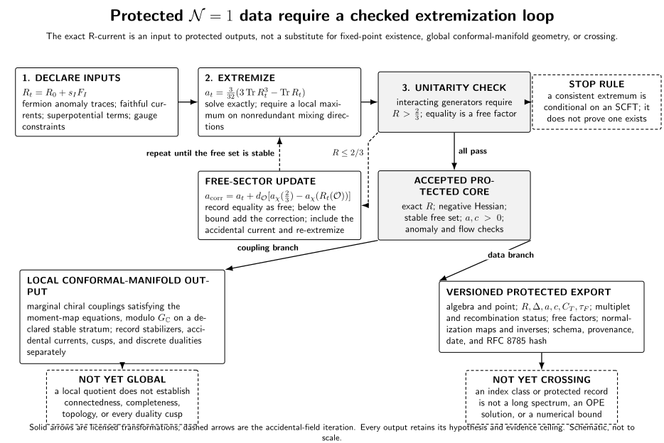
Constrained a-maximization requires a local maximum on the nonredundant current-mixing space and an iterative check of independent chiral-ring generators. A generator at $R=2/3$ is a free factor and must be separated; a value below $2/3$ requires the free-chiral correction and re-extremization. A stable free set licenses protected $R$, dimension, anomaly, and central-charge data conditional on the existence of the SCFT. The two lower branches are deliberately separate: a moment-map quotient gives local coupling-space information, while a versioned record exports only named protected data. The schematic does not establish global conformal-manifold geometry, a complete operator spectrum, crossing, or a numerical bound. Select the figure for full-size inspection. Read the machine-readable calculation record.

Boundary: polynomial-superpotential deformations

Turning on

$$W_k=g_k\operatorname{Tr}X^{k+1}$$

defines a distinct, genuinely deformed problem. At a candidate fixed point with $g_k\ne0$, superpotential marginality and the gauge-anomaly constraint require

$$R(X)=\frac{2}{k+1}, \qquad y=1-\frac{2x}{k+1}.$$

The one-parameter $W=0$ extremization above therefore cannot simply be relabeled as the deformed answer. The deformation must be relevant at the starting fixed point, the resulting fixed point must be established independently, and the chiral-ring scan must be restarted. The adjoint F-term truncates the independent dressed tower; for $SU(N_c)$, traceless variation gives $X^k$ proportional to the identity rather than literally $X^k=0$. Any newly free operators still require their own accidental-current corrections.

Iterative algorithm

1. List all anomaly-free abelian currents and impose the gauge-anomaly and superpotential constraints.
2. Declare a finite candidate set of independent four-dimensional gauge-invariant chiral-ring generators, with relations, branches, and multiplicities explicit.
3. Construct $a_t(s)$ using fermion charges and find every real stationary point exactly when possible.
4. Check the Hessian on the allowed mixing space and retain only local maxima.
5. Evaluate every declared chiral generator and identify the set $\mathcal F$ at or below $R=2/3$; record equality as a free factor rather than an interacting pass.
6. For every operator below the bound, add the free-field correction with its relations and multiplicity and re-extremize; retain operators at equality explicitly in the free sector even when their correction vanishes at that point.
7. Stop only when the maximizing branch and the free set are both unchanged. If candidate sets cycle, distinct branches demand incompatible corrections, or no consistent local maximum remains, change variables or report the method inconclusive rather than forcing a result.
8. Verify $a,c>0$, anomaly matching, superpotential marginality, and $a_{\mathrm{UV}}>a_{\mathrm{IR}}$ for the flow. State any large-rank, branch, or operator-sector truncation next to the result.

Exact rational or algebraic answers should remain exact. A decimal extremum can hide a missed root or a nearly flat direction. Product-group examples in which several gauge couplings and mixing directions must be followed simultaneously are analyzed in Barnes, Intriligator, Wecht, and Wright 2005, §§3–4.

Hessian degeneracies and marginal couplings

If the Hessian has a zero direction, first remove redundant or null current combinations and verify that every remaining current multiplet is genuinely conserved. In a unitary SCFT, a nonzero conserved flavor current has positive two-point norm, so the a-maximization Hessian is strictly negative along its mixing direction. A surviving zero mode therefore signals invalid or incomplete mixing data, not an exactly marginal coupling.

Exactly marginal couplings live in a different vector space: marginal chiral operators subject to beta-function constraints and broken-current redundancies. Their tangent and global continuation must be analyzed as on the conformal-manifold page. At a special locus a current can reappear, so the correct mixing basis and quotient slice can change; one a-maximization problem need not cover every stratum or cusp.

What the result determines

Once the exact R-symmetry is known, protected quantities follow:

$$\Delta(\mathcal O)=\frac32R(\mathcal O)$$

for chiral primaries, and

$$\begin{aligned} a&=\frac{3}{32}(3\operatorname{Tr}R^3-\operatorname{Tr}R),\\ c&=\frac{1}{32}(9\operatorname{Tr}R^3-5\operatorname{Tr}R). \end{aligned}$$

Flavor-current two-point coefficients are also related to $\operatorname{Tr}RF_IF_J$ after normalization. These outputs do not determine generic long-multiplet dimensions or OPE coefficients.

Common pitfalls

Extremizing before imposing gauge and superpotential constraints. This admits currents that are not conserved and produces meaningless stationary points.

Accepting a stationary point without the Hessian. The physical solution is a local maximum on the nonredundant mixing space.

Clamping an operator to $R=2/3$ without re-extremizing. Decoupling introduces an accidental current and changes the anomaly function for every remaining mixing parameter.

Reading a Hessian zero as a conformal-manifold tangent. The Hessian acts on flavor-current mixing directions, not on marginal couplings. Project out invalid currents and analyze exactly marginal operators separately.

Exercises

Consider a trial chiral operator with $R_{\mathcal O}(s)=1/2+s$ and multiplicity one. Write its free-field correction and evaluate it at $s=0$.

Solution

The correction is

$$\Delta a(s)=a_\chi\!\left(\frac23\right) -a_\chi\!\left(\frac12+s\right).$$

At $s=0$,

$$a_\chi\!\left(\frac12\right) =\frac{3}{32}\left[3\left(-\frac12\right)^3 +\frac12\right] =\frac{3}{256},$$

so

$$\Delta a(0)=\frac{1}{48}-\frac{3}{256} =\frac{7}{768}.$$

The positive correction replaces the inconsistent interacting assignment by the larger free-field contribution. The full theory must then be re-extremized; adding this number after the fact is not sufficient when $R_{\mathcal O}$ depends on $s$.

Verify the one-step extensive decoupling

For the leading-$N_f^2$, $x=6$ adjoint-SQCD example:

1. select the physical uncorrected stationary point from the Hessian;
2. decide whether $M_1$ is interacting or free there;
3. repeat the check for $M_1$ and $M_2$ at the corrected stationary point; and
4. state why this does not finish the finite-rank analysis.

Solution

The uncorrected Hessians are $\pm6\sqrt{719}$, so the minus branch

$$y_0^-=\frac{77-2\sqrt{719}}{71}$$

is the local maximum. It gives

$$R_t(M_1)=2y_0^-\simeq0.65836<\frac23,$$

so all $N_f^2$ components of $M_1$ belong to the free sector. After their correction is included, the physical branch again has negative Hessian,

$$y_1^-=\frac{159-2\sqrt{4647}}{69}, \qquad \widetilde a_1''(y_1^-)=-2N_f^2\sqrt{4647}.$$

At this point,

$$R_t(M_1)\simeq0.65688<\frac23, \qquad R(M_2)\simeq0.76880>\frac23.$$

Thus the leading extensive meson free set is stable after one re-extremization. The conclusion is not a complete finite-rank result because $\operatorname{Tr}X^j$, dressed baryons, chiral-ring relations, and other multiplicity-$O(1)$ sectors were omitted; some trace operators also cross the bound.

References

• Barnes, Edwin, Kenneth Intriligator, Brian Wecht, and Jason Wright. “N=1 RG Flows, Product Groups, and a-Maximization.” Nuclear Physics B 716 (2005): 33–64. arXiv:hep-th/0502049.
• Intriligator, Kenneth, and Brian Wecht. “The Exact Superconformal R-Symmetry Maximizes $a$.” Nuclear Physics B 667 (2003): 183–200. arXiv:hep-th/0304128.
• Kutasov, David, Andrei Parnachev, and David A. Sahakyan. “Central Charges and $U(1)_R$ Symmetries in $\mathcal N=1$ Super Yang–Mills.” Journal of High Energy Physics 11 (2003): 013. arXiv:hep-th/0308071.