Line Operators, Global Forms, and Discrete Theta Data

A gauge algebra and a value of $\tau$ do not yet define a globally complete $\mathcal N=4$ theory. One must decide which Wilson–’t Hooft lines are genuine, which are attached to surfaces, which bundles enter the path integral, and which discrete topological phase weights those bundles. For $\mathfrak{su}(N)$ these choices admit a particularly explicit finite-lattice description.

Required background. The $\mathcal N=4$ theory card supplies the local action. Genuine line spectra and discrete theta data supplies the global-theory criterion used here.

Helpful background. Electric–magnetic charge lattices and global form derives Abelian dualization with integral fluxes. Electric and magnetic one-form symmetries explains the background fields detected by line operators.

Wilson–’t Hooft charge classes

A Wilson line is labeled by an electric weight and an ’t Hooft line by a magnetic cocharacter. Before screening and center reduction, the pair therefore lives in a weight–coweight lattice, modulo the simultaneous Weyl action. Adjoint fields screen electric root charges; quotienting the electric weights by roots and the magnetic weights by coroots leaves the finite center classes. For a fixed algebra $\mathfrak{su}(N)$, they can be written

$$(e,m)\in\mathbb Z_N\times\mathbb Z_N.$$

We put the electric entry first and freeze the antisymmetric pairing as

$$\langle(e_1,m_1),(e_2,m_2)\rangle =e_1m_2-m_1e_2\pmod N.$$

Transporting the second line once around the first gives the phase

$$\exp\!\left[\frac{2\pi i}{N}(e_1m_2-m_1e_2)\right],$$

which must be unity for a mutually local set. A complete spectrum of genuine charge classes is therefore a maximal isotropic subgroup $L\subset\mathbb Z_N^2$: the pairing vanishes on $L$, and no further independent class can be added while retaining mutual locality. Because the pairing on $\mathbb Z_N^2$ is nondegenerate, $|L|\leq N$; a maximal isotropic subgroup has exactly $N$ elements. The weight–coweight classification and its Dirac condition are developed in Kapustin 2006, §§2–4 and Aharony, Seiberg, and Tachikawa 2013, §§1.1–1.2.

The word “genuine” is essential. A line charged under a gauged one-form symmetry may require a topological surface ending on it. Such a line is a useful relative defect but is not an isolated operator of the four-dimensional theory.

The SU(N)/ℤₖ family

Let $k$ divide $N$ and set $k'=N/k$. On a spin four-manifold, the theory conventionally denoted

$$\left(SU(N)/\mathbb Z_k\right)_n, \qquad n\in\mathbb Z_k,$$

has the genuine charge subgroup

$$L_{k,n} = \left\langle (k,0),\ (n,k') \right\rangle \subset\mathbb Z_N^2.$$

The first generator is the smallest genuine purely electric class. The second is a minimally magnetic line dressed by electric charge $n$. Their pairing is $kk'=N$, hence zero modulo $N$, and $L_{k,n}$ contains $N$ charge classes. This realizes a maximal isotropic subgroup.

The limiting cases are instructive:

global theory	generators of $L$	interpretation
$SU(N)$	$(1,0)$	all center Wilson classes are genuine
$(SU(N)/\mathbb Z_N)_0$	$(0,1)$	a purely magnetic generator is genuine
$(SU(N)/\mathbb Z_N)_n$	$(n,1)$	the minimal magnetic line is dyonically dressed

The integer $n$ records the line-spectrum and topological-phase choice. It changes the genuine dyonic line even though the perturbative adjoint-field Lagrangian is unchanged. A $2\pi$ shift of the ordinary theta angle can permute the values of $n$; only the part not reachable by such shifts is an independent discrete theta-like parameter. A systematic derivation appears in Aharony, Seiberg, and Tachikawa 2013, §§2.3–2.4.

For the smallest example, $\mathfrak{su}(2)$ has three maximal choices:

$$\begin{aligned} L_{SU(2)}&=\{(0,0),(1,0)\},\\ L_{SO(3)_+}&=\{(0,0),(0,1)\},\\ L_{SO(3)_-}&=\{(0,0),(1,1)\}. \end{aligned}$$

These theories share the same local fields but have different genuine probes.

What a complete theory card contains

For the present chapter, the minimum global theory data are

$$\mathfrak T =\bigl( \mathfrak g,\ G,\ \tau,\ L,\ \eta_{\rm disc},\ \mathcal G^{(1)},\ \mathcal A_{1\text{-form}}; \text{spacetime class and counterterms} \bigr).$$

Here $G$ fixes the allowed bundles and Wilson representations; $L$ fixes the complete mutually local genuine-line spectrum; $\eta_{\rm disc}$ fixes discrete topological phases; and $\mathcal A_{1\text{-form}}$ records the response to background two-form gauge fields, including any anomaly or local counterterm choice. In the $\mathfrak{su}(N)$ theories above, the one-form symmetry acting faithfully on the genuine charge classes is the Pontryagin dual $\mathcal G^{(1)}\simeq\operatorname{Hom}(L,U(1))$, although whether it is called electric, magnetic, or dyonic depends on the embedding $L\subset\mathbb Z_N^2$ Gaiotto et al. 2015, §§4–5.

Neither $G$ nor $L$ alone is always sufficient. On a spin four-manifold the subgroup $L_{k,n}$ captures the familiar $(SU(N)/\mathbb Z_k)_n$ choices, but coupling to background fields can require a quadratic refinement and a specified local counterterm. On a non-spin manifold, line statistics and the allowed topological phases require additional data. Every duality arrow must declare the domain in which its theory card is complete.

Modular transport of the lattice

Use

$$\tau'=\frac{a\tau+b}{c\tau+d}, \qquad \begin{pmatrix}e'\\m'\end{pmatrix} = \begin{pmatrix}a&-b\\-c&d\end{pmatrix} \begin{pmatrix}e\\m\end{pmatrix}.$$

Because the matrix has determinant one, two independent charges $(e_i,m_i)$ and their transformed charges $(e'_i,m'_i)$, for $i=1,2$, obey

$$e'_1m'_2-m'_1e'_2 =e_1m_2-m_1e_2\pmod N,$$

so mutual locality is preserved. Define $\rho(M)(e,m)^T=(e',m')^T$ by the displayed charge matrix. The transformed subgroup $L'=\rho(M)L$ defines the target theory. For the generators

$$S:\tau\mapsto-\frac1\tau,\quad(e,m)\mapsto(m,-e),$$ $$T:\tau\mapsto\tau+1,\quad(e,m)\mapsto(e-m,m).$$

The sign in the $T$ action is the passive convention of this chapter. In the common active convention the line is transformed in the opposite direction and the electric shift has the opposite sign.

For $\mathfrak{su}(2)$, reduction modulo two gives

$$S:\quad SU(2)\longleftrightarrow SO(3)_+, \qquad SO(3)_-\longmapsto SO(3)_-,$$

and

$$T:\quad SU(2)\longmapsto SU(2), \qquad SO(3)_+\longleftrightarrow SO(3)_-.$$

Thus $S$ is not an internal symmetry of the $SU(2)$ theory with its standard Wilson spectrum: it points to the $SO(3)_+$ theory. A modular word is a loop only if its final line subgroup and discrete data agree with its initial values.

The same convention makes the Witten effect on the general family explicit. Since $T$ sends the magnetic generator $(n,k')$ to $(n-k',k')$,

$$T:\quad L_{k,n}\longmapsto L_{k,n-k'}.$$

Thus a $2\pi$ shift of $\theta$ can move between distinct theory cards. The shift orbit has length $k/\gcd(k,k')$; equivalently, the invariant residue $n\bmod\gcd(k,k')$ labels the distinct orbits that cannot be connected by the ordinary theta shift. At the level of these spin-manifold line spectra, the minimal shift that returns $L_{k,n}$ to itself is

$$\Delta\theta_L =2\pi\frac{k}{\gcd(k,k')}$$

on the stated spin-manifold domain. Extra background counterterms can further refine the transformation of the complete theory card. The primary source often uses the active convention, for which the same line-lattice relation reads $n\mapsto n+k'$.

For $S$, one can compute the target rather than merely assert that it exists. Let $d=\gcd(k,n)$ and choose integers $e_0,m_0$ with

$$e_0k+m_0n=d.$$

Then

$$S:\quad \left(SU(N)/\mathbb Z_k\right)_n \longrightarrow \left(SU(N)/\mathbb Z_{k_S}\right)_{n_S}, \qquad k_S=\frac{N}{d}, \qquad n_S\equiv-m_0k'\pmod{k_S}.$$

Changing the Bézout pair changes $n_S$ only by the equivalences of the target lattice. In particular, $n=0$ gives $k_S=k'=N/k$ and $n_S=0$; the special case $k=1$ exchanges $SU(N)$ with $PSU(N)_0$. For composite $N$, the full set of theory cards need not form one $SL(2,\mathbb Z)$ orbit; a common divisor of all electric and magnetic classes is preserved. This is why an orbit diagram must show the actual lattices, not just a ring of global-form names Aharony, Seiberg, and Tachikawa 2013, §2.4.

The diagram below makes the rank-one case concrete. Read the left panel first to see which screened charge classes are genuine, then follow the source-labeled $S$ and $T$ arrows in the middle panel. The torus panel explains why the same passive transformation preserves both the intersection pairing and the BPS norm.

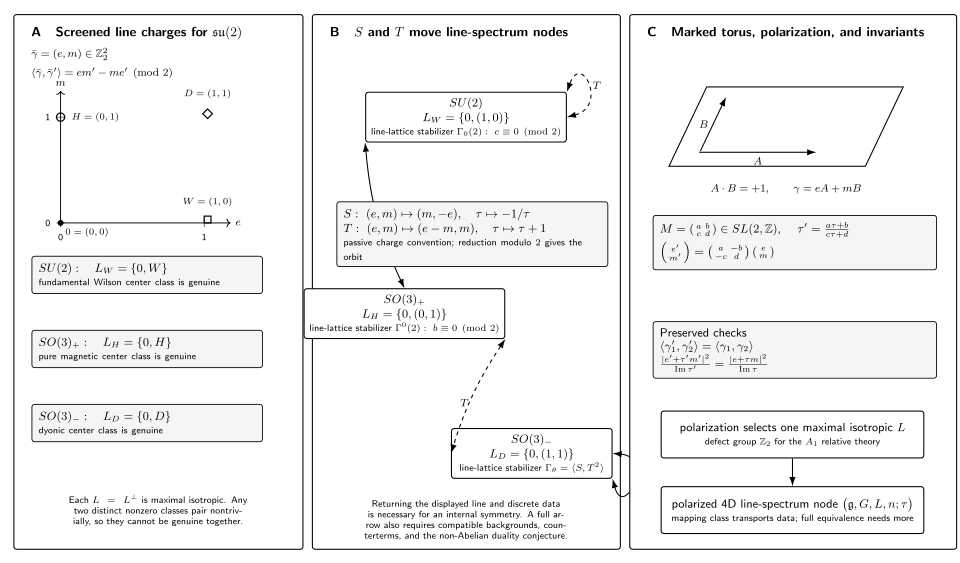
On a spin four-manifold, the three maximal-isotropic subgroups of $\mathbb Z_2^2$ select $SU(2)$, $SO(3)_+$, and $SO(3)_-$. The solid $S$ arrows and dashed $T$ arrows give exact transport of $\tau$ and the screened genuine-line lattice in the chapter’s passive convention; only a node’s line-lattice stabilizer can be an internal modular subgroup, and only after the remaining background and counterterm data also return. The marked-torus panel shows the geometric origin of the same charge map after a polarization is chosen. This is a schematic, not-to-scale classification: exact lattice transport does not by itself prove the conjectured equivalence of all non-Abelian observables. Select the figure for full-size inspection, or read the structured charge-lattice and orbit record (JSON).

One-form symmetry and background dependence

Genuine lines are charged objects for one-form global symmetries. Gauging an electric subgroup changes the global gauge group and introduces magnetic sectors; a discrete theta term can produce a mixed electric–magnetic anomaly. The background-field formulation of these operations is given in Gaiotto et al. 2015, §§4–6.

This background dependence is physically measurable. Partition functions on manifolds with nontrivial two-cycles can be resolved by ’t Hooft flux. Surface operators can detect whether a line is genuine, and interfaces must say how one-form backgrounds are transmitted. Local correlators of adjoint operators on $\mathbb R^4$ generally miss this information.

Scope and refinements

The finite $\mathbb Z_N^2$ description records charges after adjoint screening; it does not replace the full weight and coweight labels of individual line operators. Operator ordering, monopole bubbling, spin, and supersymmetric dressing add further data.

The formula $L_{k,n}$ is stated for spin four-manifolds, appropriate to a theory with fermions. On non-spin manifolds, line spins, quadratic refinements, and theta periodicities can change the classification. Background two-form fields can also reveal anomalies invisible in the bare subgroup $L$.

For a non-simply-laced algebra, electric and magnetic root systems differ in length and the Langlands-dual algebra need not equal the original algebra. The naive $SL(2,\mathbb Z)$ action must then be replaced by the appropriate subgroup and lacing-number transformation.

Exercises

1. Check isotropy. Prove that any two elements of $L_{k,n}$ have vanishing Dirac pairing modulo $N$.

Solution

Write the two elements as $(a_1k+b_1n,b_1k')$ and $(a_2k+b_2n,b_2k')$. Their pairing is $(a_1b_2-b_1a_2)kk'=(a_1b_2-b_1a_2)N$, which vanishes modulo $N$.

2. Recover the three $\mathfrak{su}(2)$ theories. Evaluate $L_{k,n}$ for $(k,n)=(1,0),(2,0),(2,1)$.

Solution

For $(1,0)$ the generator is $(1,0)$, giving $SU(2)$. For $(2,0)$ the nonzero generator is $(0,1)$, giving $SO(3)_+$. For $(2,1)$ it is $(1,1)$, giving $SO(3)_-$.

3. Find the line-spectrum theta period. For $N=12$ and $k=4$, determine the number of $2\pi$ shifts required to return $L_{k,n}$ to itself.

Solution

Here $k'=N/k=3$. Each passive $T$ shift changes $n$ by $-3$ modulo $4$. Since $\gcd(4,3)=1$, four shifts are required, and the fixed-card theta period is $8\pi$.

4. Compute a nontrivial $S$ target. Apply the displayed Bézout formula to $(SU(4)/\mathbb Z_2)_1$.

Solution

$d=\gcd(2,1)=1$, so $k_S=4$. Choose $e_0=0$ and $m_0=1$, and note that $k'=2$. Then $n_S\equiv-2\equiv2\pmod4$. Therefore

$$S:\quad(SU(4)/\mathbb Z_2)_1\longrightarrow(PSU(4))_2.$$

Directly, $S$ sends the generators $(2,0)$ and $(1,2)$ to $(0,2)$ and $(2,3)$ modulo four; these generate the same subgroup as $(2,1)$, the $L_{4,2}$ target.

References

• Aharony, Ofer, Nathan Seiberg, and Yuji Tachikawa. “Reading between the Lines of Four-Dimensional Gauge Theories.” Journal of High Energy Physics 08 (2013): 115. doi:10.1007/JHEP08(2013)115.
• Gaiotto, Davide, Anton Kapustin, Nathan Seiberg, and Brian Willett. “Generalized Global Symmetries.” Journal of High Energy Physics 02 (2015): 172. doi:10.1007/JHEP02(2015)172.
• Kapustin, Anton. “Wilson–’t Hooft Operators in Four-Dimensional Gauge Theories and S-Duality.” Physical Review D 74 (2006): 025005. doi:10.1103/PhysRevD.74.025005.