Matter, Higher Rank, and Integrable-System Structures

For rank $r>1$, Seiberg–Witten geometry retains the same core structure: an $r$-complex-dimensional special Kähler base, an integral electromagnetic local system, and singular loci where charged states can become massless. In many Lagrangian families these data come from a genus-$r$ curve and its Jacobian; in others the physical torus is a Prym variety or another $r$-dimensional abelian subvariety of a higher-genus Jacobian. The precise curve and integrable-system realization depend on the gauge group, matter, ultraviolet construction, and global data. Rank alone does not determine a universal spectral curve.

Required background. Curves, differentials, and periods supplies the construction, while singularities and monodromies supplies the global constraints. Helpful background. Product groups and quiver dynamics illustrates why matter and quiver structure alter the answer.

Pure SU(N) as the basic higher-rank family

For pure $SU(N)$, introduce

$$P_N(x)=x^N-\sum_{k=2}^{N}u_kx^{N-k},$$

where $u_k$ have scaling dimension $k$ in the semiclassical region. A standard hyperelliptic presentation is

$$y^2=P_N(x)^2-\Lambda^{2N}.$$

For generic moduli this curve has genus

$$g=N-1=\operatorname{rank}SU(N).$$

One convenient differential is proportional to

$$\lambda_{\mathrm{SW}} =x\,d\log\!\left( \frac{P_N(x)-y}{P_N(x)+y} \right),$$

with the overall factor fixed by the weak-coupling normalization. Equivalent forms such as $xP_N'(x)dx/y$ can differ by constants and exact terms after the curve equation is used.

Choose $N-1$ $A$ cycles and $N-1$ $B$ cycles. Their periods give

$$a^I=\oint_{A^I}\lambda_{\mathrm{SW}}, \qquad a_{D,I}=\oint_{B_I}\lambda_{\mathrm{SW}}.$$

At weak coupling, the $a^I$ approach Cartan eigenvalue differences. The exact coupling matrix is the genus-$N-1$ period matrix in the special basis. Pure-$SU(N)$ curves and their period and monodromy tests are derived in Klemm, Lerche, Theisen, and Yankielowicz 1995, §§2–4.

An explicit genus-two test: pure SU(3)

Set

$$P_3(x)=x^3-u_2x-u_3, \qquad y^2=\bigl(P_3(x)-\Lambda^3\bigr) \bigl(P_3(x)+\Lambda^3\bigr).$$

The two cubic factors have discriminants

$$\Delta_+=4u_2^3-27(u_3+\Lambda^3)^2, \qquad \Delta_-=4u_2^3-27(u_3-\Lambda^3)^2.$$

Their resultant contributes the remaining scale factor, so the degree-six polynomial has discriminant

$$\operatorname{Disc}_x(P_3^2-\Lambda^6) =64\Lambda^{18}\Delta_+\Delta_-.$$

Thus the singular locus is not a set of isolated points but two cusped curves in the $(u_2,u_3)$ plane. Their cusps occur at

$$(u_2,u_3)=(0,-\Lambda^3), \qquad (u_2,u_3)=(0,+\Lambda^3),$$

where one cubic factor develops a triple root. These are stronger degenerations than a generic point of either discriminant component: two intersecting cycles can vanish, so a mutually local one-hypermultiplet description is insufficient. This mutually nonlocal degeneration is the pure-$SU(3)$ origin of the original fixed-point construction Argyres and Douglas 1995, §§2–4.

The two components also meet where

$$u_3=0, \qquad u_2^3=\frac{27}{4}\Lambda^6.$$

For nonzero $\Lambda$ there are three $\mathbb Z_3$-related intersection points in the complex base; the positive-real one has $u_2=3\Lambda^2/2^{2/3}$. At such a transverse intersection, the two cubic factors develop double roots at distinct $x$ values. The local fiber has two separated nodes and the corresponding local vanishing cycles can be chosen disjoint, so their intersection pairing is zero. This is topologically different from either cusp, where three branch points collide and the two local vanishing cycles intersect.

There is also a useful nonsingular real checkpoint. For $\Lambda>0$, $u_2=3\Lambda^2$, and $u_3=0$, all six branch points are real:

$$\frac{x}{\Lambda}\approx -1.879385, -1.532089, -0.347296, +0.347296, +1.532089, +1.879385.$$

Three real cuts can join adjacent pairs, but only two encircling cycles are independent; their two dual cycles complete a symplectic basis of $H_1(\Sigma_2,\mathbb Z)$. Following those branch points toward a discriminant component makes the associated vanishing cycle geometrically visible.

The figure puts the discriminant divisor and the regular genus-two fiber side by side. On the left, compare a smooth point of a component, a transverse component intersection, and a cusp; on the right, count the independent cycles rather than the three planar cuts.

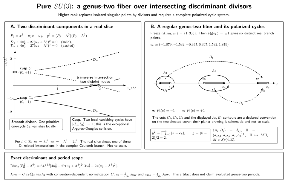
For $y^2=P_3^2-\Lambda^6$, the left panel shows a real slice of the two complex discriminant divisors, including their cusps and one of three $\mathbb Z_3$-related transverse intersections. The right panel freezes $\Lambda=1$, $u_2=3$, $u_3=0$ and declares one schematic cut-and-cycle convention for the six exact branch roots. The discriminant, roots, intersection matrix, and dimensional checks are quantitative; the planar contours are not to scale, the differential normalization remains conventional, and no numerical genus-two period matrix is claimed. See the structured SU(3) record.

Adding fundamental matter

For $SU(N)$ with $N_f$ fundamental hypermultiplets in an asymptotically free range, a common schematic family is

$$y^2=P_N(x)^2 -\Lambda^{2N-N_f}\prod_{f=1}^{N_f}(x+m_f),$$

with shifts of $P_N$, mass conventions, and extra factors depending on $N_f$ and the chosen normalization. The differential has poles whose residues encode $m_f$.

Three checks fix the physical interpretation:

1. $[\lambda_{\mathrm{SW}}]=1$ and $[m_f]=1$;

2. residues reproduce integral flavor charges in the central charge;

3. decoupling $m_{N_f}\to\infty$ with

   $$\Lambda_{N_f-1}^{\,2N-(N_f-1)} =m_{N_f}\Lambda_{N_f}^{\,2N-N_f}$$

   held fixed recovers the lower-flavor family.

At conformal $N_f=2N$, the gauge coupling is dimensionless and the curve depends on a modular parameter rather than only a dimensional transmutation scale. The asymptotically free formula should not be extended there without the correct modular completion.

Algebraic integrable systems

An algebraic completely integrable system has a complex symplectic total space fibered by abelian varieties. The Coulomb moduli are base coordinates; the Jacobian or Prym variety of the spectral curve supplies the torus fiber. The gauge-theory curve as the fiber of an integrable system is developed in Donagi and Witten 1996, §§2–4. Special coordinates are action variables,

$$a^I=\oint_{A^I}p\,dq,$$

and the Seiberg–Witten differential plays the role of the Liouville one-form $p\,dq$.

For pure $SU(N)$ theory, the relevant classical system is the periodic Toda chain. Its spectral equation can be written

$$z+\frac{\Lambda^{2N}}{z}=2P_N(x),$$

which becomes the hyperelliptic curve after eliminating $z$. The Toda Hamiltonians map to the Coulomb invariants $u_k$.

This is more than a resemblance of equations: the spectral curve, symplectic form, action variables, and weak-coupling limits agree. The Toda-chain realization and exact-solution correspondence are exhibited in Gorsky, Krichever, Marshakov, Mironov, and Morozov 1995, pp. 466–474. But the map is family-specific. It does not imply that every $\mathcal N=2$ theory is governed by the periodic Toda chain.

Other established correspondences

Different ultraviolet theories lead to different systems:

• $\mathcal N=2^*$ $SU(N)$ theory is related to an elliptic Calogero–Moser system;
• certain linear quivers lead to spin chains or Hitchin systems;
• class-S theories are organized by Hitchin systems on punctured curves;
• five- and six-dimensional lifts lead to relativistic or doubly elliptic variants.

For each statement, specify the gauge/matter family, compactification, punctures, masses, coupling parameters, and the precise spectral differential. Similarity of a polynomial is not enough to establish an integrable-system realization.

Singular fibers in higher rank

The discriminant is a divisor with multiple components. At a generic point on one component, one primitive cycle vanishes and a mutually local hypermultiplet can become massless. At intersections, several cycles vanish.

If all pairings vanish,

$$\langle\gamma_i,\gamma_j\rangle=0,$$

one can choose a common electric frame and obtain a weakly coupled multi-hypermultiplet description. If some pairing is nonzero, a single local abelian Lagrangian fails and an interacting fixed point can appear.

The local monodromy matrices lie in $Sp(2r,\mathbb Z)$. Their product around a large loop must match semiclassical Weyl and logarithmic monodromy. Higher rank adds path-order complexity: discriminant components can braid, and matrices for different vanishing cycles need not commute.

Polarization and global form

The curve supplies $H_1(\Sigma,\mathbb Z)$ with its integral intersection form. After the Seiberg–Witten polarization is specified, this is a natural computational lattice for periods and dynamical BPS charges. It must nevertheless be distinguished from the ultraviolet lattice of genuine line operators. Global form and a discrete theta angle select a mutually local set of center-valued Wilson–’t Hooft charges; equivalently, one obtains an integral line lattice between the appropriate root–coroot and weight–coweight lattices. The finite quotient that measures the mismatch is a defect or one-form-symmetry group, not automatically another symplectic charge lattice.

For a nonprincipal polarization of type $D=\operatorname{diag}(d_1,\ldots,d_r)$, an adapted basis has pairing matrix

$$J_D= \begin{pmatrix} 0&D\\ -D&0 \end{pmatrix},$$

rather than the unimodular matrix with $D=\mathbf 1$. Consequently, matching genus and complex period matrices does not establish equality of line spectra. One must state which integral cycles represent dynamical particles, how ultraviolet Wilson–’t Hooft lines embed, and which finite quotient records the global-form choice. The charge-lattice discussion develops the same distinction in rank one.

A bounded verification workflow

For a proposed higher-rank curve:

1. verify genus equals the Coulomb rank on the generic fiber;
2. check dimensions, discrete symmetries, and weak-coupling factorization;
3. fix $\lambda_{\mathrm{SW}}$ by periods and flavor residues;
4. derive the one-loop coupling matrix asymptotically;
5. test massive-flavor decoupling;
6. compute discriminant components and vanishing-cycle pairings;
7. verify integral symplectic monodromies and their global product;
8. identify the exact integrable system and map its Hamiltonians and symplectic form;
9. state exceptional loci and any conjectural extension separately.

Passing only the genus and symmetry checks leaves many inequivalent geometries.

Common pitfalls

Calling every spectral curve an established integrable system. The action variables, symplectic form, and Hamiltonian map must also be identified.

Using the asymptotically free matter curve at $N_f=2N$. The conformal coupling and modular dependence require a different normalization.

Equating the Jacobian lattice with the physical line lattice automatically. Global form and polarization can select a different integral structure.

Exercises

For pure $SU(3)$, write $P_3(x)=x^3-u_2x-u_3$ and $f(x)=P_3(x)^2-\Lambda^6$.

1. Factor $f$ into two cubics and derive its discriminant, including the resultant between the factors.
2. Locate the two cusps of the discriminant locus. What happens to the branch points and vanishing cycles there?
3. At $\Lambda=1$, $u_2=3$, $u_3=0$, order the six real branch points and describe a cut system with the correct number of independent $A$ and $B$ cycles.

Solution

The factorization is

$$f=(P_3-\Lambda^3)(P_3+\Lambda^3).$$

The cubic discriminants are $\Delta_+=4u_2^3-27(u_3+\Lambda^3)^2$ and $\Delta_-=4u_2^3-27(u_3-\Lambda^3)^2$. At a root of $P_3-\Lambda^3$, the other factor equals $2\Lambda^3$, so the resultant has magnitude $(2\Lambda^3)^3=8\Lambda^9$. The product rule for discriminants therefore gives

$$\operatorname{Disc}_x f =64\Lambda^{18}\Delta_+\Delta_-.$$

The cusps are $(u_2,u_3)=(0,-\Lambda^3)$ and $(0,+\Lambda^3)$. At the first, $P_3-\Lambda^3=x^3$; at the second, $P_3+\Lambda^3=x^3$. Three branch points coincide. Two independent neighboring vanishing cycles can then have nonzero intersection, which is why the cusp is not described by two mutually local free hypermultiplets.

For the stated real slice, the ordered roots are approximately

$$-1.879385, -1.532089, -0.347296, +0.347296, +1.532089, +1.879385.$$

Join adjacent pairs to make three cuts. Small loops around all three cuts sum to zero in homology, so choose any two as $A_1,A_2$ and choose two sheet-changing paths as dual $B^1,B^2$. The degree-six hyperelliptic curve has genus two and therefore precisely two independent $A$ periods and two independent $B$ periods.

References

• Argyres, Philip C., and Michael R. Douglas. “New Phenomena in $SU(3)$ Supersymmetric Gauge Theory.” Nuclear Physics B 448 (1995): 93–126. DOI; Open PDF.
• Donagi, Ron, and Edward Witten. “Supersymmetric Yang–Mills Theory and Integrable Systems.” Nuclear Physics B 460 (1996): 299–334. arXiv:hep-th/9510101.
• Gorsky, Anton, Igor Krichever, Andrei Marshakov, Alexei Mironov, and Andrei Morozov. “Integrability and Seiberg–Witten Exact Solution.” Physics Letters B 355 (1995): 466–474. arXiv:hep-th/9505035.
• Klemm, Albrecht, Wolfgang Lerche, Stefan Theisen, and Stefan Yankielowicz. “Simple Singularities and $\mathcal N=2$ Supersymmetric Yang–Mills Theory.” Physics Letters B 344 (1995): 169–175. arXiv:hep-th/9411048.