Instanton Counting and the Omega Background

The Omega background turns the framed-instanton integral on $\mathbb C^2$ into an equivariant integral. For a four-dimensional $\mathcal N=2$ $U(N)$ theory at generic equivariant and Coulomb parameters, the resolved ADHM space has isolated torus fixed points labeled by $N$ -tuples of Young diagrams. The exact instanton factor is then a fixed-point sum, but only after the framing, stability chamber, tangent-space orientation, instanton fugacity, mass shifts, and treatment of Abelian factors have been fixed.

Required background. Use finite-dimensional equivariant localization and the field-theoretic instanton zero-mode analysis.

Helpful background. The Seiberg–Witten curve and periods provide the undeformed low-energy quantity recovered from the small-Omega limit.

Equivariant data of the Omega background

The convention card on this page is the cohomological, four-dimensional calculation for framed $U(N)$ instantons on $\mathbb C^2$ . K-theoretic five-dimensional counting exponentiates the weights below and is not obtained by changing notation alone.

Write $\mathbb R^4\simeq\mathbb C^2$ with coordinates $(z_1,z_2)$ . The rotation torus acts by

(t_1,t_2)\mathbin{\cdot}(z_1,z_2) =(t_1z_1,t_2z_2).

Writing $t_i=e^{i\vartheta_i}$ , the parameters $\epsilon_i$ below are the additive infinitesimal weights. They have mass dimension one; they are not the dimensionless angles $\vartheta_i$ . After the rotations are combined with R-symmetry and gauge transformations, the localizing differential has the schematic square

Q_\Omega^2 =\epsilon_1J_{12}+\epsilon_2J_{34} +\sum_{\alpha=1}^{N}a_\alpha G_\alpha +\sum_f m_fF_f.

The Coulomb parameters $a_\alpha$ , equivariant masses $m_f$ , and $\epsilon_{1,2}$ are all additive torus weights. Framing fixes a trivialization at infinity. Consequently, the Cartan of the framing group acts equivariantly instead of being divided out as an ordinary global gauge zero mode. Nekrasov’s construction realizes the instanton measure as precisely such an equivariant integral Nekrasov 2003, §§2.2 and 3.1–3.4.

The instanton partition function is graded by instanton number:

Z_{\mathrm{inst}}(q_{\rm UV}) =\sum_{k\geq0}q_{\rm UV}^{k} Z_k, \qquad q_{\rm UV}=e^{2\pi i\tau}.

For an asymptotically free theory, $q_{\rm UV}$ is replaced by the appropriate power of the strong scale after a renormalization convention is chosen. A sector-dependent sign is also conventional: below we use a common arm–leg factor for which the combinatorial fugacity is $\mathfrak q=(-1)^{N-1}q_{\rm UV}$ . Moving this phase between $\mathfrak q$ and the fixed-point Euler class changes no physics, but mixing the two conventions changes every odd-instanton coefficient.

Framed ADHM space and its stability chamber

For $U(N)$ instanton number $k$ , introduce vector spaces $V\simeq\mathbb C^k$ and $W\simeq\mathbb C^N$ and maps

B_1,B_2\in\operatorname{End}(V), \qquad I\in\operatorname{Hom}(W,V), \qquad J\in\operatorname{Hom}(V,W).

They obey the complex and real moment-map equations

[B_1,B_2]+IJ=0, \qquad [B_1,B_1^\dagger]+[B_2,B_2^\dagger] +II^\dagger-J^\dagger J=\zeta\,\mathbf 1_V,

followed by the $U(k)$ quotient. With the displayed sign and $\zeta>0$ , stability says that no proper subspace $S\subsetneq V$ may contain $\operatorname{im}I$ while satisfying $B_1S,B_2S\subset S$ . This is a convention-sensitive statement: reversing the real moment map reverses the stability chamber.

At $\zeta=0$ , pointlike instantons make the quotient singular. Taking $\zeta\ne0$ , equivalently using the framed torsion-free-sheaf compactification or a noncommutative resolution, produces the smooth space on which the equivariant integral is defined. The resolution is not decorative ultraviolet language; it decides which compactification boundary and residues enter the answer Nekrasov 2003, §§3.1–3.6.

The torus acts on $(B_1,B_2,I,J)$ and on the framing space. Its isolated fixed points are

\vec Y=(Y_1,\ldots,Y_N), \qquad |\vec Y|=\sum_{\alpha}|Y_\alpha|=k.

For generic $(a_\alpha,\epsilon_1,\epsilon_2)$ these fixed points are isolated. If Coulomb or equivariant weights collide, the fixed locus need not remain zero-dimensional and the simple inverse-Euler-class formula must be replaced by localization on the resulting component. The Young-diagram classification and the fixed-point weights are derived in Nekrasov 2003, §§3.5–3.7.

Tangent weights and the fixed-point sum

For a box $s=(i,j)$ in a Young diagram $Y$ , define arm and leg lengths

A_Y(s)=Y_i-j, \qquad L_Y(s)=Y_j^T-i.

Set $\epsilon_+=\epsilon_1+\epsilon_2$ and $a_{\alpha\beta}=a_\alpha-a_\beta$ . One convenient cohomological convention packages the additive tangent weights into the Nekrasov factor

\begin{aligned} \mathcal N_{Y,W}(x) ={}&\prod_{s\in Y} \left[x+\epsilon_1\bigl(A_Y(s)+1\bigr)-\epsilon_2L_W(s)\right] \\ &\times\prod_{t\in W} \left[x-\epsilon_1A_W(t)+\epsilon_2\bigl(L_Y(t)+1\bigr)\right]. \end{aligned}

With the fugacity phase declared above, the pure-vector sum is

Z_{\mathrm{inst}}^{\rm pure} =\sum_{\vec Y} \mathfrak q^{|\vec Y|} \prod_{\alpha,\beta=1}^{N} \mathcal N_{Y_\alpha,Y_\beta}(a_{\alpha\beta})^{-1}, \qquad \mathfrak q=(-1)^{N-1}q_{\rm UV}.

This is the inverse equivariant Euler class of the ADHM tangent complex, not an arbitrary product assigned to a diagram. The two products in $\mathcal N$ are the paired deformation and obstruction weights; their arm–leg asymmetry records which $\mathbb C$ plane carries $\epsilon_1$ and which carries $\epsilon_2$ .

For $N_f$ fundamental hypermultiplets, choose the equivariant-mass convention in which

Z_{\rm fund}(\vec a,\vec Y;\vec m) =\prod_{f=1}^{N_f}\prod_{\alpha=1}^{N} \prod_{(i,j)\in Y_\alpha} \left[a_\alpha+m_f+\epsilon_1(i-1)+\epsilon_2(j-1)\right].

Other representations are Euler classes of different associated bundles and should not be inferred from this formula. In many physical-mass conventions the symbol called $m_f$ differs from this equivariant mass by $\epsilon_+/2$ , with the sign fixed by the R-symmetry and Dirac-operator convention. This is the common source of an apparently missing half-shift.

A non-Abelian one-instanton benchmark

At $k=1$ , exactly one color $\alpha$ carries $Y_\alpha=[1]$ and every other diagram is empty. Evaluating the arm–leg factors and including the declared fugacity phase gives

Z_1^{U(N),N_f} =\frac{1}{\epsilon_1\epsilon_2} \sum_{\alpha=1}^{N} \frac{\displaystyle\prod_{f=1}^{N_f}(a_\alpha+m_f)} {\displaystyle\prod_{\beta\ne\alpha} a_{\alpha\beta}(a_{\alpha\beta}+\epsilon_+)}.

This is Nekrasov’s $Z_1=(\epsilon_1\epsilon_2)^{-1}\sum_\alpha S_\alpha(0)$ , with $S_\alpha$ specialized to fundamental matter Nekrasov 2003, eqs. (3.21) and (3.23). It tests four pieces at once: the self-weight $\epsilon_1\epsilon_2$ , both Coulomb-difference factors, the matter numerator, and the sector orientation.

For pure $SU(2)$ set $a_1=a$ , $a_2=-a$ . The two colored boxes give

Z_1^{SU(2),\rm pure} =\frac{2}{\epsilon_1\epsilon_2 \left(4a^2-\epsilon_+^2\right)}.

Therefore $\epsilon_1\epsilon_2 Z_1\to1/(2a^2)$ as $\epsilon_{1,2}\to0$ . A different phase convention for the strong scale can flip the displayed odd-instanton sign, but it must flip both the fixed-point series and the Seiberg–Witten expansion. The poles at $a_{\alpha\beta}=0$ or $a_{\alpha\beta}=-\epsilon_+$ also have a clear meaning: the assumed isolated-fixed-point description has degenerated.

For framed $U(1)$ the same calculation gives

Z_1^{U(1)}=\frac1{\epsilon_1\epsilon_2}.

This coefficient belongs to the resolved ideal-sheaf or noncommutative problem. Smooth finite-action instantons do not exist in ordinary commutative $U(1)$ gauge theory on $\mathbb R^4$ , so interpreting it as an ordinary Abelian instanton would change the problem being counted.

Controlled limits

In the convention used by Nekrasov’s original fixed-point series, the instanton prepotential is

\mathcal F_{\mathrm{inst}}(a,m,q) =\lim_{\epsilon_1,\epsilon_2\to0} \epsilon_1\epsilon_2\log Z_{\mathrm{inst}},

with a simultaneous scaling $\epsilon_i=\lambda\widehat\epsilon_i$ at fixed nonzero ratio,

\log Z_{\mathrm{inst}} =\frac{\mathcal F_{\mathrm{inst}}}{\epsilon_1\epsilon_2} +o(\lambda^{-2}).

Subleading terms need not be $O(1)$ ; they can scale as $\lambda^{-1}$ . Some references reverse the leading sign by reversing one equivariant orientation, so the defining asymptotic equation, not the symbol $\mathcal F_{\mathrm{inst}}$ , decides the translation. The limit is collective: it is taken after summing diagrams or controlling their thermodynamic asymptotics, at fixed Coulomb parameters away from singular loci. Nekrasov and Okounkov prove the connection between the partition sum and Seiberg–Witten geometry in this limit Nekrasov and Okounkov 2006, §§3–4.

For the Nekrasov–Shatashvili limit, first declare the full Nekrasov factor being used. In the convention

Z_{\mathrm{Nek}}=Z_{\mathrm{pert}}Z_{\mathrm{inst}},

with any decoupled normalization removed separately, one takes

\epsilon_2\to0, \qquad \widetilde W_{\mathrm{eff}} =\lim_{\epsilon_2\to0} \epsilon_2\log Z_{\mathrm{Nek}},

and obtains a two-dimensional effective twisted superpotential. Using $Z_{\mathrm{inst}}$ alone gives only its instanton contribution. The result retains $\epsilon_1$ as the quantization parameter and is not the undeformed four-dimensional prepotential Nekrasov and Shatashvili 2009, §3.1, eq. (3.7). The specialization $\epsilon_1=-\epsilon_2$ is yet another operation; it simplifies the measure but does not send the Omega deformation to zero.

The right branch of the shared map places this calculation alongside, but does not identify it with, localized sphere integrals and protected traces. Follow it from the framed equivariant moduli problem through isolated fixed points and tangent weights to the Nekrasov series, then inspect the stability, mass-shift, Abelian-factor, convergence, and limiting data that must travel into any comparison.

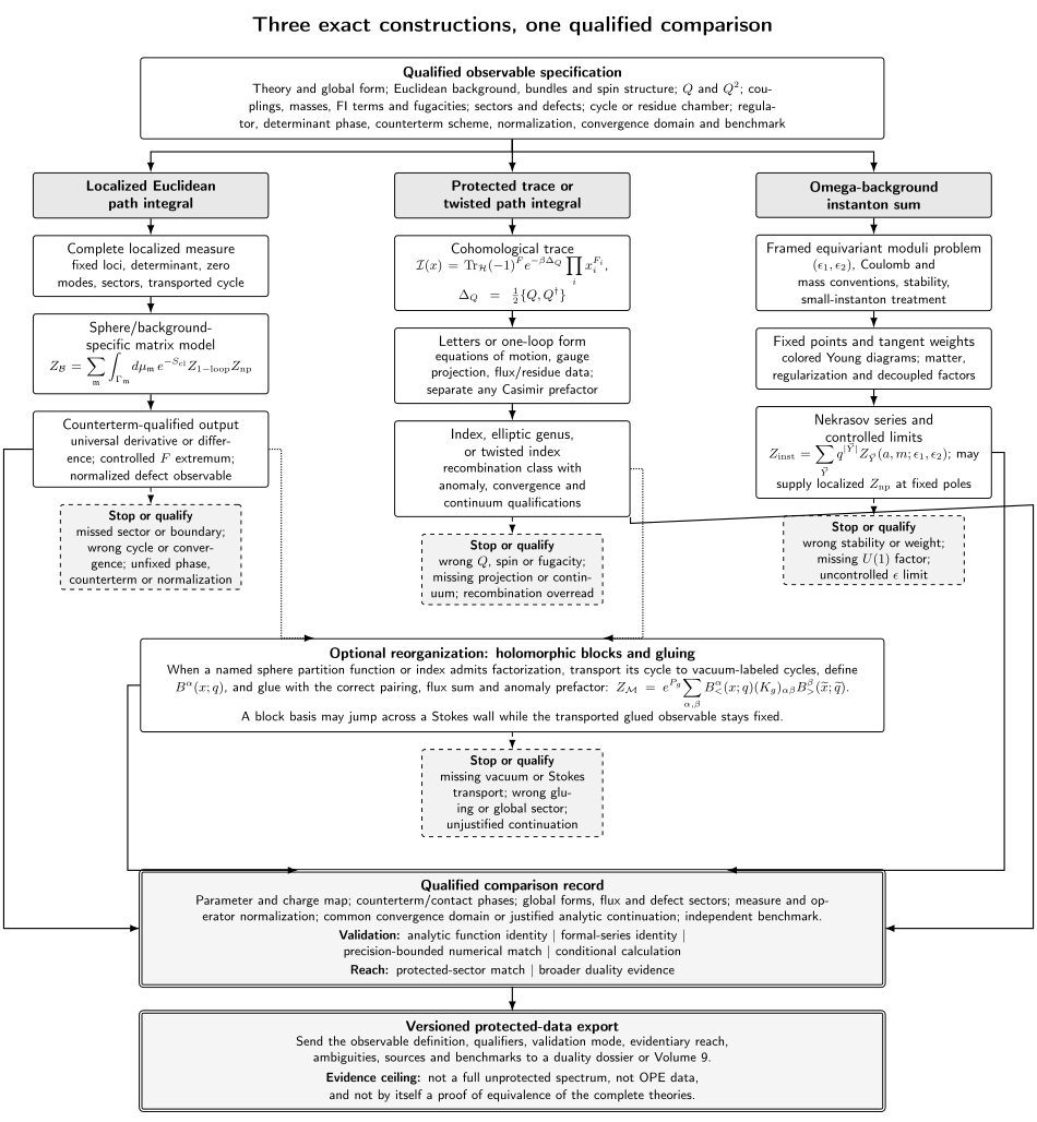
The instanton branch starts from a framed, resolved moduli problem with declared $(\epsilon_1,\epsilon_2)$ , Coulomb and mass conventions, global gauge data, stability chamber, and small-instanton treatment. Only then do fixed points and tangent weights define the Young-diagram series and its controlled prepotential or Nekrasov–Shatashvili limits. On a compact background such as $S^4$ , these fixed-point functions can instead supply the localized branch’s pole factors $Z_{\mathrm{np}}$ once the local equivariant and mass conventions are matched. The dashed exit marks a wrong chamber or tangent weight, an omitted $U(1)$ or decoupled factor, a hidden mass shift, and an uncontrolled equivariant limit. Convergence with the other branches occurs only in a qualified comparison record; it does not assert that they compute the same object. The map is schematic and not to scale.

The reflowing text equivalent of the exact-observable map preserves every branch, failure exit, comparison field, and evidence limit for narrow-screen and print reading.

Failure modes

Changing the resolved problem. Setting $\zeta$ to zero before integration reintroduces the small-instanton singularity. A framed sheaf compactification, noncommutative resolution, and contour prescription are related descriptions only after their chambers and boundary contributions are matched.

Changing stability silently. Reversing the moment-map sign or crossing an ADHM or contour wall can change which residues represent the integral.

Hiding the Euler-class orientation. The phase $(-1)^{N-1}$ may be placed in the instanton fugacity or in each fixed-point sector. Using the arm–leg formula from one convention and the $q$ definition from another fails already at $k=1$ .

Mixing $U(N)$ and $SU(N)$ . The constraint $\sum_\alpha a_\alpha=0$ does not by itself remove every decoupled Abelian factor from matter or correspondence formulas.

Ignoring mass shifts. Equivariant and physical hypermultiplet masses often differ by $(\epsilon_1+\epsilon_2)/2$ .

Using a degenerate torus action. Coincident $a_\alpha$ or special relations among $a_{\alpha\beta}$ and $\epsilon_i$ can make the fixed locus non-isolated. A formula derived for isolated points cannot simply be evaluated there term by term.

Taking a singular limit term by term. Individual partitions can diverge as $\epsilon_{1,2}\to0$ even when $\log Z$ has a controlled collective asymptotic expansion.

Assuming convergence from formal counting. The fixed- $k$ equivariant integral and the all- $k$ power series are different questions. State whether $Z_{\rm inst}$ is used as a formal series in $q$ , as a convergent function in a domain, or through analytic continuation.

Exercises

1. Derive the colored one-box weight

For pure $U(N)$ , put one box in $Y_\alpha$ and leave the other diagrams empty. Derive the $\alpha$ term in $Z_1$ , including the fugacity phase.

Solution

The self-pair gives $\mathcal N_{[1],[1]}(0)=\epsilon_1\epsilon_2$ . For each $\beta\ne\alpha$ ,

\mathcal N_{[1],\varnothing}(a_{\alpha\beta}) =a_{\alpha\beta}+\epsilon_+, \qquad \mathcal N_{\varnothing,[1]}(a_{\beta\alpha}) =-a_{\alpha\beta}.

The product therefore contributes $(-1)^{N-1}\prod_{\beta\ne\alpha}a_{\alpha\beta}(a_{\alpha\beta}+\epsilon_+)$ . The one-instanton fugacity $\mathfrak q=(-1)^{N-1}q_{\rm UV}$ cancels that orientation sign, leaving

\frac{1}{\epsilon_1\epsilon_2} \prod_{\beta\ne\alpha} \frac{1}{a_{\alpha\beta}(a_{\alpha\beta}+\epsilon_+)}.

2. Check the pure SU(2) prepotential coefficient

Set $a_1=a$ , $a_2=-a$ in the one-instanton formula and take $\epsilon_{1,2}\to0$ after summing the two fixed points.

References

Section titled “References”- Nekrasov, N. A. “Seiberg–Witten Prepotential from Instanton Counting.” Advances in Theoretical and Mathematical Physics 7 (2003): 831–864. DOI; Open PDF.
- Nekrasov, N., and A. Okounkov. “Seiberg–Witten Theory and Random Partitions.” In The Unity of Mathematics, 525–596. Boston: Birkhäuser, 2006. DOI; Open PDF.
- Nekrasov, N. A., and S. L. Shatashvili. “Quantization of Integrable Systems and Four Dimensional Gauge Theories.” arXiv:0908.4052 [hep-th] (2009). arXiv; Open PDF.
Further reading
Section titled “Further reading”- Tachikawa, Y. “A Review on Instanton Counting and W-Algebras.” arXiv:1412.7121 [hep-th] (2014). arXiv.
Original QFT.org content:CC BY 4.0, unless an item supplies different terms. Third-party material retains its own terms.