Wheeler–DeWitt Cosmology: Boundary Conditions, Inner Products, and Probabilities

A Wheeler–DeWitt solution is not yet a probability distribution for a universe. One must also declare the operator and its domain, the physical product, a frequency sector or another positivity prescription, a clock, and the observable being conditioned on. In the flat FLRW model with a massless scalar, those choices can be made sharply enough that group averaging, positive-frequency Klein–Gordon flux, and scalar-clock quantum mechanics become unitarily equivalent. The equivalence is exact inside that declared model; it does not make cosmological probabilities independent of ordering, measure, clock, or boundary prescription.

Required background. Minisuperspace Reductions and Approximation Control supplies the truncation and its omitted-mode limits. Wheeler–DeWitt Quantization and the Problem of Time supplies the general constraint.

Helpful background. Bilinear and Hermitian Forms, Adjoints, and Isometries and Self-Adjointness, Extensions, and Unitary Evolution supply the mathematical controls.

From the reduced constraint to a hyperbolic equation

Work on the sector $a>0$ and define dimensionless coordinates

$$\alpha=\ln\frac{a}{a_\star}, \qquad \varphi=\frac{\phi}{\sqrt6M_{\mathrm{Pl}}}, \qquad p_\alpha=ap_a, \qquad p_\varphi=\sqrt6M_{\mathrm{Pl}}p_\phi.$$

Here $a_\star>0$ is an arbitrary reference scale, $V_0$ is the fiducial comoving coordinate volume, $M_{\mathrm{Pl}}=(8\pi G)^{-1/2}$, and $p_a,p_\phi$ are the canonical momenta.

Multiplying the classical Hamiltonian constraint by the positive function $12V_0M_{\mathrm{Pl}}^2a^3$ gives

$$\mathcal C_0=p_\varphi^2-p_\alpha^2\approx0.$$

This multiplication preserves the classical constraint surface for $a>0$, but doing it before quantization is a choice: a different densitization can change the quantum measure and domain. For the baseline calculation, choose

$$\begin{aligned} \widehat{\mathcal C}_0 &=-\partial_\varphi^2+\partial_\alpha^2,\\ \widehat\Theta &=-\partial_\alpha^2, &D(\widehat\Theta)&=H^2(\mathbb R), &\mathcal H_\alpha&=L^2(\mathbb R,d\alpha). \end{aligned}$$

The non-negative self-adjoint operator $\widehat\Theta$ has the square root $\widehat H=\sqrt{\widehat\Theta}=|\widehat p_\alpha|$. We define the site’s positive-$p_\varphi$ sheet by the first-order equation

$$-i\partial_\varphi\Psi=\widehat H\Psi.$$

This explicit equation is safer than the phrase “positive frequency”: with these conventions its modes contain $e^{+ik\varphi}$, opposite to a common QFT time-dependence convention. Craig and Singh use this same sign in their solvable FLRW treatment; after $x=\ln\nu=3\alpha+\text{constant}$ and $\varphi=\phi/(\sqrt6M_{\mathrm{Pl}})$, their wave equation and measure become the equations here, up to an overall normalization Craig and Singh 2010, § III.B, Eqs. (3.17)–(3.31), Open PDF.

Frequency and expansion are different signs

Let $k>0$, $\sigma=\operatorname{sgn}p_\varphi$, and $s=\operatorname{sgn}p_\alpha$. The four generalized plane-wave solutions are

$$u_{k,\sigma,s}(\alpha,\varphi) =\frac{e^{i\sigma k\varphi+isk\alpha}}{\sqrt{4\pi k}}, \qquad \sigma,s\in\{+1,-1\}.$$

They are delta-normalized modes, not normalizable universe states. The classical momentum is

$$p_\alpha=-6V_0M_{\mathrm{Pl}}^2a^3H_{\mathrm{FLRW}},$$

for positive lapse. Thus $s=-1$ is expanding and $s=+1$ is contracting. On the positive-$p_\varphi$ sheet, Hamilton’s equations also give

$$\frac{d\alpha}{d\varphi} =-\frac{p_\alpha}{p_\varphi}=-s.$$

To orient the conserved current, use the superspace metric and current

$$G^{AB}=\operatorname{diag}(+1,-1), \qquad J^A=-\frac{i}{2}\Psi^* \overleftrightarrow{\partial^A}\Psi.$$

For one plane wave,

$$J^\varphi=p_\varphi|u|^2, \qquad J^\alpha=-p_\alpha|u|^2, \qquad \partial_AJ^A=0.$$

The diagram separates the two binary choices. Inspect the vertical component to read the scalar-frequency sheet and the horizontal component to read expansion or contraction.

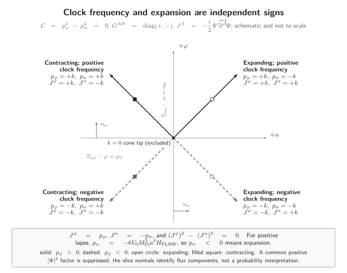
Four branches of $\mathcal C_0=p_\varphi^2-p_\alpha^2=0$ with $J^A=(p_\varphi,-p_\alpha)|u|^2$. All four rays have $k>0$; the cone tip is excluded. A constant-$\varphi$ slice distinguishes the sign of $p_\varphi$; it cannot distinguish expanding from contracting geometry. The schematic is not to scale, and neither a physical product nor a clock prescription is selected by the drawing.

Open the full-size SVG · Download the semantic record

The same information is available without the figure:

Frequency sign and geometric branch are independent labels

Scalar momentum	Scale momentum	Clock current	Scale current	Proper-time geometry	Klein–Gordon sheet sign
pϕ = +k	pα = −k	Jϕ > 0	Jα > 0	Expanding	Positive
pϕ = +k	pα = +k	Jϕ > 0	Jα < 0	Contracting	Positive
pϕ = −k	pα = −k	Jϕ < 0	Jα > 0	Expanding	Negative
pϕ = −k	pα = +k	Jϕ < 0	Jα < 0	Contracting	Negative

Both expanding and contracting modes therefore have positive constant-$\varphi$ flux on the chosen sheet. The unrestricted Klein–Gordon form is indefinite because it includes both values of $\sigma$, not because it includes both geometric branches. This distinction is central to the exact left/right and frequency decomposition in Craig and Singh 2010, § III.B, Eqs. (3.19)–(3.31), Open PDF.

WKB branches and their control

Now allow a real potential in

$$\widehat\Theta=-\partial_\alpha^2+U(\alpha), \qquad (\partial_\varphi^2+\widehat\Theta)\Psi=0.$$

For a stationary component $e^{i\omega\varphi}\chi_\omega(\alpha)$ on the chosen sheet, take $\omega>0$ and define

$$K_\omega(\alpha)=\sqrt{\omega^2-U(\alpha)}.$$

Where $K_\omega^2>0$, define the leading WKB residual

$$\mathcal R_{\mathrm{WKB}} =\left| \frac{3(K_\omega')^2}{4K_\omega^4} -\frac{K_\omega''}{2K_\omega^3} \right|.$$

The leading branches are controlled when $\mathcal R_{\mathrm{WKB}}\ll1$. A convenient stronger check is to require both $|K_\omega'|/K_\omega^2\ll1$ and $|K_\omega''|/K_\omega^3\ll1$. In that regime,

$$\begin{aligned} \Psi_{\omega,E} &\simeq \frac{C_E}{\sqrt{2K_\omega}} \exp\!\left(i\omega\varphi-i\int^\alpha K_\omega(\alpha')\,d\alpha'\right),\\ \Psi_{\omega,C} &\simeq \frac{C_C}{\sqrt{2K_\omega}} \exp\!\left(i\omega\varphi+i\int^\alpha K_\omega(\alpha')\,d\alpha'\right). \end{aligned}$$

The amplitude follows from leading current conservation. With the orientation above, the scale currents are $J_E^\alpha\simeq+|C_E|^2/2$ and $J_C^\alpha\simeq-|C_C|^2/2$. At a turning point $K_\omega=0$, the residual ceases to be small; reflection can mix the branches, so separately conserved expanding and contracting probabilities are no longer licensed. WKB flux is a useful semiclassical diagnostic, but it becomes a probability only after a product, state, coarse graining, and conditioning rule are supplied Halliwell 1991, § 7, especially Eqs. (7.13)–(7.20), Open PDF.

For the free benchmark below, $U=0$, so $K_\omega=\omega$, $\mathcal R_{\mathrm{WKB}}=0$, and these WKB branches are exact. The three products can therefore be compared on the same expanding/contracting decomposition.

Three products on one frequency sheet

Group averaging starts from an auxiliary test state $f$ and the self-adjoint constraint:

$$\eta(f)=\int_{-\infty}^{\infty}\frac{d\lambda}{2\pi} e^{i\lambda\widehat{\mathcal C}_0}f.$$

With unitary Fourier conventions, its induced product is

$$\langle\eta f,\eta g\rangle_{\mathrm{ind}} =\int dp_\varphi\,dp_\alpha\, \delta(p_\varphi^2-p_\alpha^2) \overline{\widetilde f}\,\widetilde g.$$

Resolving the delta function on the positive-$p_\varphi$ sheet gives

$$\langle\eta f,\eta g\rangle_{\mathrm{ind},+} =\sum_{s=\pm1}\int_0^\infty\frac{dk}{2k} \overline{F_s(k)}G_s(k), \qquad F_s(k)=\widetilde f(k,sk).$$

The cone tip $k=0$ is excluded here; a state with support there needs a separate infrared treatment. Define $A_s(k)=F_s(k)/\sqrt{2k}$ and the covariantly normalized representative

$$\Psi_{\mathrm{KG}} =\sum_{s=\pm1}\int_0^\infty dk\, A_s(k)u_{k,+,s}.$$

Then

$$\begin{aligned} \langle\eta f,\eta g\rangle_{\mathrm{ind},+} &=\sum_s\int_0^\infty dk\,\overline{A_s}B_s,\\ (\Psi_1,\Psi_2)_{\mathrm{KG}} &=-i\int_{-\infty}^{\infty}d\alpha\, \Psi_1^*\overleftrightarrow{\partial_\varphi}\Psi_2 =\sum_s\int_0^\infty dk\,\overline{A_s}B_s. \end{aligned}$$

Finally apply the spectral Newton–Wigner map

$$\psi_{\mathrm{NW}}=(2\widehat H)^{1/2}\Psi_{\mathrm{KG}}.$$

It changes the covariant $1/\sqrt{2k}$ mode normalization into the ordinary Fourier normalization. On any constant-$\varphi$ slice,

$$\langle\psi_1,\psi_2\rangle_{\mathrm{Sch}} =\int_{-\infty}^{\infty}d\alpha\, \psi_1^*(\alpha,\varphi_0)\psi_2(\alpha,\varphi_0) =\sum_s\int_0^\infty dk\,\overline{A_s}B_s.$$

The formulas are unitarily equivalent, not literally the same formula applied to the same raw wavefunction. Hartle and Marolf compare the Klein–Gordon and induced products in reparametrization-invariant systems Hartle and Marolf 1997, §§ II.C–III.B, Open PDF. Group averaging additionally assumes a self-adjoint constraint, a suitable dense test space, a meaningful group integral, and positivity of the induced form Giulini 2000, §§ 2–5, Eqs. (6)–(15), Open PDF.

What each product does—and what makes the three descriptions equivalent

Description	Domain used here	Sign	Required rematching	Failure condition
Klein–Gordon flux	Covariantly normalized solutions on a constant-scalar slice	Positive on one declared frequency sheet; indefinite on both sheets	Orient the slice and fix the frequency sign	No stable frequency split, nonzero boundary flux, or an invalid slice
Group-averaged induced product	Rigging-map image of a chosen test space	Positive direct sum when the averaging construction succeeds	Resolve the mass-shell measure, including its 1/(2k) weight	Non-self-adjoint constraint, divergent average, bad test space, or unresolved cone tip
Scalar-clock Schrödinger product	Newton–Wigner representative on one good clock patch	Positive	Select a sheet and apply the square-root spectral map	Clock turning point, multiple intersections, or a generator/domain not transformed with the clock

On both scalar-frequency sheets, the induced product is a positive direct sum. The raw Klein–Gordon form instead assigns opposite signs to the two sheets. No choice of expanding versus contracting branch repairs that unrestricted sign.

An exact two-branch probability benchmark

Plane waves are unsuitable for probabilities, so choose a normalized spectral profile

$$g_\kappa(k)=\frac{2k}{\kappa^{3/2}}e^{-k/\kappa}, \qquad \kappa>0, \qquad \int_0^\infty dk\,|g_\kappa(k)|^2=1.$$

For a concrete state, take

$$A_{-}(k)=\frac{\sqrt3}{2}g_\kappa(k), \qquad A_{+}(k)=\frac12g_\kappa(k),$$

where $s=-1$ is expanding and $s=+1$ is contracting. Orthogonality of their disjoint $p_\alpha$ supports gives the exact spectral-projector probabilities

$$P_E=\int_0^\infty dk\,|A_-(k)|^2=\frac34, \qquad P_C=\int_0^\infty dk\,|A_+(k)|^2=\frac14.$$

The positive-$p_\varphi$ Klein–Gordon flux, the induced product, and the scalar-clock product all give these same weights after the maps above. The result has no Monte Carlo or discretization uncertainty: it is an analytic benchmark. Its uncertainty is structural instead—the state weights were chosen, the homogeneous model was truncated, and the operator, measure, clock, and frequency sheet were fixed.

The Newton–Wigner wavefunction is also elementary. Define

$$f_\kappa(x)= \sqrt{\frac{2\kappa}{\pi}}\frac{1}{(1+i\kappa x)^2}.$$

Then

$$\psi(\alpha,\varphi) =\frac{\sqrt3}{2}f_\kappa(\alpha-\varphi) +\frac12f_\kappa^*(\alpha+\varphi).$$

The branch components are orthogonal in momentum space, although their local configuration-space density can interfere. Probabilities in the scale factor include the Jacobian

$$dP=\frac{da}{a} \left|\psi\!\left(\ln\frac{a}{a_\star},\varphi\right)\right|^2.$$

At every finite $\varphi$, this packet tends pointwise to zero as $a\to0$. Nevertheless, as $\varphi\to-\infty$, its expanding component moves to $\alpha\to-\infty$, and the probability below any fixed low-volume threshold approaches its full branch weight $3/4$. Pointwise vanishing at the singular frontier is therefore not a history-level singularity criterion. In the standard flat-FLRW Wheeler–DeWitt quantization, Craig and Singh instead find that the decoherent history entering an arbitrarily fixed small-volume interval in at least one of the limits $\varphi\to\pm\infty$ has probability one for every physical state Craig and Singh 2010, § V.D, Eqs. (5.20)–(5.34), Open PDF.

Ordering and measure stress test

The baseline measure $d\alpha=da/a$ corresponds to $q=-1$ in the exact family

$$\mathcal H_q=L^2((0,\infty),a^q\,da), \qquad \Theta_q=-a^{-q}\partial_a \!\left(a^{q+2}\partial_a\right).$$

The map

$$(U_q\psi)(\alpha)=a^{(q+1)/2}\psi(a)$$

is unitary from $\mathcal H_q$ to $L^2(\mathbb R,d\alpha)$. Take $D(\Theta_q)=U_q^{-1}H^2(\mathbb R)$. Then $\Theta_q$ is the self-adjoint operator unitarily equivalent to

$$U_q\Theta_qU_q^{-1} =-\partial_\alpha^2+\frac{(q+1)^2}{4}.$$

This one calculation exposes three different questions.

• Normalization. If the state and mass-shell weight are rematched, the induced measure becomes $dk/(2\omega_q)$ with $\omega_q(k)=\sqrt{k^2+(q+1)^2/4}$, and the normalized branch weights remain $3/4$ and $1/4$. Reusing a wavefunction with the wrong measure is not a comparison of normalized states.
• Dynamics. Retaining the constant term is a genuine ordering change. A narrow packet moves with $|d\alpha/d\varphi|=k/\omega_q(k)$ rather than unit speed, and long-time phases also change. Ordering effects are small only for a packet concentrated where $(q+1)^2/(4k^2)\ll1$, over a time interval short enough that phase errors remain controlled. Subtracting the constant instead defines a representation-equivalent family.
• Singular-frontier behavior. The original representative is $\psi_q(a)=a^{-(q+1)/2}(U_q\psi)(\alpha)$. Its pointwise limit can change from zero to divergent as $q$ changes while the Hilbert-space norm stays finite. The bare statement “the wavefunction vanishes at $a=0$” is therefore not measure invariant.

Factor ordering can alter the differential operator, current, scalar product, and near-singularity behavior in more general minisuperspace models Šteigl and Hinterleitner 2006, §§ 4–6.3, especially Eqs. (26), (33), (35)–(38), and (41)–(55), Open PDF. Our family supplies an exact adversary, not a proof that all orderings reduce to a constant shift.

Clock stress test

A monotonic relabeling is harmless only when the generator and event labels are transformed with it. For $\tau=\lambda\varphi$, $\lambda>0$,

$$-i\partial_\tau\Psi=\frac{\widehat H}{\lambda}\Psi, \qquad \tau=\lambda\varphi.$$

Comparing the same events then gives the same probability. Keeping $\widehat H$ instead would move the packet $\lambda$ times too far while preserving its norm; normalization alone does not establish clock equivalence.

The nonlinear candidate $\chi=\varphi^2$ fails more sharply:

$$\{\chi,\mathcal C_0\}=4\varphi p_\varphi.$$

It is tangent to the gauge flow at $\varphi=0$, and every value $\chi>0$ intersects an orbit at both signs of $\varphi$. A conditional probability at fixed $\chi$ is ambiguous until an additional sign branch and its weighting are supplied. Using $\alpha$ as a clock instead requires one sign of $p_\alpha$ and fails at a WKB turning point, so it is not global for the two-branch packet or a reflected state. Clock-dependent domains and qualitatively different evolution occur in broader cosmological models Gielen and Menéndez-Pidal 2022, §§ 3–6, Open PDF; that model includes an additional fluid and serves here as an adversarial example, not a result for the pure scalar fixture.

When boundary data are actually required

In the baseline representation, $a=0$ means $\alpha=-\infty$, not $\alpha=0$. The operator $-\partial_\alpha^2$ on $H^2(\mathbb R)$ is already self-adjoint; no finite-endpoint boundary parameter is available. Whether boundary data are required must be decided after fixing the operator, measure, and domain.

For example, the half-line normal form

$$T_g=-\frac{d^2}{dx^2}+\frac{g}{x^2}$$

is limit-point at $x=0$ for $g\ge3/4$, so no boundary datum is needed there. For $g<3/4$ it is limit-circle and extension data are required; for $g<-1/4$ the inverse-square attraction also destroys semiboundedness Dereziński and Richard 2017, §§ 2.2–2.3 and Theorem 5.5, Open PDF. “There is an endpoint” is therefore not enough to infer either a unique boundary condition or a healthy quantum dynamics.

DeWitt proposed vanishing at singular geometries,

$$\lim_{a\to0}\Psi(a,\varphi)=0,$$

as a heuristic condition DeWitt 1967, Eq. (6.31), pp. 1129–1130. Depending on the representation it may be a pointwise asymptotic statement, a Dirichlet condition in a genuine half-line problem, or not invariant under a change of measure. It is not automatically a self-adjoint-extension condition, a positive probability rule, or proof that singular histories have zero probability. Modern reviews accordingly separate local wavefunction criteria from global evolution, observables, and unitarity Thébault 2023, § 4.1 and §§ 5.1–5.2, Open PDF.

What survives the tests

The strongest exact statement is conditional:

In the flat homogeneous massless-scalar model, for the fixed densitized constraint, the free full-line operator $\widehat\Theta=-\partial_\alpha^2$ on $H^2(\mathbb R)$, the positive-$p_\varphi$ sheet with $k=0$ excluded, and a valid scalar clock, the group-averaged induced, Klein–Gordon, and deparametrized products are unitarily equivalent after the $(2\widehat H)^{1/2}$ spectral rematching. Because $[\widehat H,\operatorname{sgn}(\widehat p_\alpha)]=0$ in this free model, the expanding and contracting spectral projectors have exact conserved probabilities.

The tests do not establish ordering-, measure-, boundary-, or clock-independent cosmological probabilities. They do not select the state, prove singularity resolution, control the omitted inhomogeneous modes, or define full quantum gravity. When a Wheeler–DeWitt Born–Oppenheimer branch is used to recover QFT for perturbations, the emergent time, branch control, and subleading unitarity corrections must be checked anew Brizuela, Kiefer, and Krämer 2016, §§ III–IV and VIII–IX, Open HTML.

Common pitfalls

Calling the expanding branch “positive frequency.” Frequency sign is $\operatorname{sgn}p_\varphi$; expansion is $\operatorname{sgn}p_\alpha$. They are independent labels.

Treating a conserved current as a Born density. Conservation does not imply positivity. The unrestricted Klein–Gordon form is indefinite, and a clock-conditioned density requires a declared sector and representation.

Normalizing a plane wave. The $u_{k,\sigma,s}$ are generalized eigenfunctions. Probabilities require square-integrable spectral packets such as $g_\kappa$.

Moving a boundary condition between representations. A pointwise condition, a zero-flux condition, and a self-adjoint domain are different statements. Their relation depends on the operator and measure.

Reading a state-selection proposal out of the equation. The Wheeler–DeWitt constraint admits many solutions. No-boundary and tunneling prescriptions add saddle, contour, and regularity data; the equation alone chooses neither.

Exercises

1. Current signs and classical geometry

For $u_{k,\sigma,s}$, calculate both current components and show which sign labels the proper-time geometry. Why can a constant-$\varphi$ flux not distinguish expansion from contraction?

Solution

Since $\partial^\varphi=\partial_\varphi$ and $\partial^\alpha=-\partial_\alpha$,

$$J^\varphi=\sigma k|u|^2, \qquad J^\alpha=-sk|u|^2.$$

For positive lapse, $p_\alpha=-6V_0M_{\mathrm{Pl}}^2a^3H_{\mathrm{FLRW}}$. Hence $s=-1$ is expanding and $s=+1$ is contracting, independent of $\sigma$. The normal to a constant-$\varphi$ slice measures $J^\varphi$, which depends on $\sigma$ but not $s$; it separates frequency sheets rather than geometric branches.

2. Resolve the group-averaging measure

On the positive-$p_\varphi$ sheet, resolve $\delta(p_\varphi^2-p_\alpha^2)$ and derive the $1/(2k)$ measure. Then find the map to ordinary $L^2(dk)$ amplitudes.

Solution

For fixed $p_\alpha\ne0$,

$$\delta(p_\varphi^2-p_\alpha^2) =\frac{ \delta(p_\varphi-|p_\alpha|) +\delta(p_\varphi+|p_\alpha|)}{2|p_\alpha|}.$$

Keep the first root, write $p_\alpha=sk$ with $k>0$, and sum over $s=\pm1$. This gives

$$\sum_s\int_0^\infty\frac{dk}{2k} \overline{F_s(k)}G_s(k).$$

Setting $A_s=F_s/\sqrt{2k}$ converts it to $\sum_s\int dk\,\overline{A_s}B_s$. The same factor turns the covariant mode $e^{ik\varphi+isk\alpha}/\sqrt{4\pi k}$ into the ordinary Fourier mode after applying $(2H)^{1/2}$. The derivation excludes $k=0$.

3. Transform the ordering family

Verify that $U_q$ is unitary and derive $U_q\Theta_qU_q^{-1}$. What remains invariant after correctly rematching the state, and what changes?

Solution

Because $da=a\,d\alpha$,

$$\int_0^\infty a^q\,da\,|\psi(a)|^2 =\int_{-\infty}^{\infty}d\alpha\, |a^{(q+1)/2}\psi(a)|^2,$$

so $U_q$ is unitary. Substitute $\psi=a^{-(q+1)/2}g(\alpha)$ and use $\partial_a=a^{-1}\partial_\alpha$. The first-derivative terms cancel, leaving

$$U_q\Theta_qU_q^{-1} =-\partial_\alpha^2+\frac{(q+1)^2}{4}.$$

With the correct $dk/(2\omega_q)$ mass-shell measure and normalized amplitudes, the branch weights remain $3/4$ and $1/4$. If the constant is retained, the dispersion, group speed, and phases change. The pointwise $a\to0$ behavior of the untransformed representative also changes with $q$.

4. Test the DeWitt criterion with a packet

Show that $f_\kappa(x)$ vanishes for $|x|\to\infty$, but that the expanding packet moves below every fixed threshold $\alpha_c$ as $\varphi\to-\infty$. What conclusion is ruled out?

Solution

The modulus is

$$|f_\kappa(x)|^2 =\frac{2\kappa/\pi}{(1+\kappa^2x^2)^2},$$

which tends to zero as $|x|^{-4}$. The expanding density is centered at $\alpha=\varphi$. Therefore, for every fixed $\alpha_c$,

$$\lim_{\varphi\to-\infty} \int_{-\infty}^{\alpha_c}d\alpha\, |f_\kappa(\alpha-\varphi)|^2=1.$$

In the two-branch state, the corresponding contribution approaches its weight $3/4$. Thus pointwise vanishing of the wavefunction at $a=0$ for each finite clock value does not imply zero probability for approaching the low-volume region over a relational history.

5. Break a proposed clock

For $\chi=\varphi^2$, compute its transversality factor and count the intersections of the surface $\chi=c>0$ with a generic orbit. State the missing datum in a conditional probability at fixed $\chi$.

Solution

Using $\mathcal C_0=p_\varphi^2-p_\alpha^2$,

$$\{\chi,\mathcal C_0\}=4\varphi p_\varphi.$$

It vanishes at $\varphi=0$, so the clock surface ceases to be transverse there. For $c>0$, the condition $\chi=c$ permits both $\varphi=+\sqrt c$ and $\varphi=-\sqrt c$ on the same orbit. A conditional probability needs an additional sign-of-$\varphi$ branch and a rule for its weight; conditioning on $\chi$ alone is not single valued.

Where to continue

• Quantum-Cosmology Observables and the Problem of Time develops relational observables, clock rematching, and history probabilities.
• No-Boundary and Tunneling Wavefunction Proposals adds state-selection, contour, and saddle data.
• Quantum Geometrodynamics Beyond Minisuperspace restores functional degrees of freedom and studies the Born–Oppenheimer interface with QFT.
• Semiclassical Recovery, Decoherence, Obstructions, and Status asks when WKB branches can support consistent probabilistic histories.

The chapter overview contains the structure diagram and validity and failure diagram. They are embedded there once so that their shared chapter-level context is not repeated on every article.

For the chapter-wide comparison of assumptions, counterevidence, falsifiers, and claim ceilings, see the claim-domain table.

References

• Brizuela, D., C. Kiefer, and M. Krämer. “Quantum-Gravitational Effects on Gauge-Invariant Scalar and Tensor Perturbations during Inflation: The de Sitter Case.” Physical Review D 93 (2016): 104035. DOI. Open HTML.
• Craig, D. A., and P. Singh. “Consistent Probabilities in Wheeler–DeWitt Quantum Cosmology.” Physical Review D 82 (2010): 123526. DOI. Open PDF.
• Dereziński, J., and S. Richard. “On Schrödinger Operators with Inverse Square Potentials on the Half-Line.” Annales Henri Poincaré 18 (2017): 869–928. DOI. Open PDF.
• DeWitt, B. S. “Quantum Theory of Gravity. I. The Canonical Theory.” Physical Review 160 (1967): 1113–1148. DOI.
• Gielen, S., and L. Menéndez-Pidal. “Unitarity, Clock Dependence and Quantum Recollapse in Quantum Cosmology.” Classical and Quantum Gravity 39 (2022): 075011. DOI. Open PDF.
• Giulini, D. “Group Averaging and Refined Algebraic Quantization.” Nuclear Physics B Proceedings Supplements 88 (2000): 385–388. DOI. Open PDF.
• Halliwell, J. J. “Introductory Lectures on Quantum Cosmology.” In Quantum Cosmology and Baby Universes, edited by S. Coleman, J. B. Hartle, T. Piran, and S. Weinberg, 159–243. Singapore: World Scientific, 1991. DOI. Open PDF.
• Hartle, J. B., and D. Marolf. “Comparing Formulations of Generalized Quantum Mechanics for Reparametrization-Invariant Systems.” Physical Review D 56 (1997): 6247–6257. DOI. Open PDF.
• Šteigl, R., and F. Hinterleitner. “Factor Ordering in Standard Quantum Cosmology.” Classical and Quantum Gravity 23 (2006): 3879–3894. DOI. Open PDF.
• Thébault, K. P. Y. “Big Bang Singularity Resolution in Quantum Cosmology.” Classical and Quantum Gravity 40 (2023): 055007. DOI. Open PDF.