JT/SYK Spectral Form Factors and Universality Windows

The spectral form factor is a Fourier microscope for energy differences. It can expose the two-level correlations predicted by a random-matrix symmetry class, but the familiar slope–dip–ramp–plateau outline is not itself a proof of chaos, unitarity, or a unique JT/SYK duality. The observable changes when one changes the symmetry sector, normalization, energy window, unfolding, ensemble average, or time smoother.

This page keeps those operations separate and carries out a reproducible test: a finite $q=4$, $N_\chi=14$ SYK parity block is compared with an independently generated, identically processed finite GUE ensemble. The calculation supports a deliberately narrow statement about this size, block, bulk window, first form-factor moment, and time range. Its failed controls show exactly why a stronger statement would be premature.

Required background. Random Matrices, Spectral Statistics, and Ensemble Questions supplies symmetry classes and unfolding; Spectral Statistics, Form Factors, and Late-Time Evidence supplies the general diagnostic.

Helpful background. Finite Size, Symmetry Sectors, and Scrambling False Positives develops finite-system controls; Finite-N Spectra, Recurrences, and the Late-Time Plateau explains the exact late-time ceiling.

Evidence cutoff: 29 August 2026.

One spectrum produces several form factors

Let $j$ label a disorder realization or matrix draw, and restrict the trace to one irreducible symmetry block $\mathcal H_\alpha$:

$$Z_j(s)=\operatorname{Tr}_{\mathcal H_\alpha}e^{-sH_j} =\sum_{n\in\mathcal H_\alpha}e^{-sE_{jn}}.$$

The annealed thermal form factor, its disconnected part, and its connected part are

$$K_{\rm ann}(\beta,t) =\left\langle \left\lvert Z_j(\beta+it)\right\rvert^2\right\rangle_j,$$ $$K_{\rm disc}(\beta,t) =\left\lvert\left\langle Z_j(\beta+it)\right\rangle_j\right\rvert^2, \qquad K_{\rm conn}=K_{\rm ann}-K_{\rm disc}.$$

Here $\langle\cdot\rangle_j$ is an average over independently drawn Hamiltonians. Expanding the first expression while retaining that average gives

$$K_{\rm ann}(\beta,t) =\left\langle \sum_{m,n}e^{-\beta(E_{jm}+E_{jn})} e^{-it(E_{jm}-E_{jn})} \right\rangle_j.$$

Several operations are often hidden behind the same overbar. They are not interchangeable.

Operation	What is acted on	What it answers
Disorder or matrix average	Independent Hamiltonians $H_j$	What is typical in the declared ensemble?
Time smoothing	One time series, through a stated kernel $\mathcal S_\sigma$	What trend remains after suppressing fluctuations on scale $\sigma$?
Energy filtering	Levels weighted by a stated $w(E-E_0)$	Which spectral band contributes to the observable?
Unfolding	Coordinates $E\mapsto\xi=\overline N(E)$	What remains after removing a declared smooth density?

Only the first operation creates the ensemble-connected covariance above. A fixed realization has the noisy quantity $\lvert Z_1\rvert^2$; applying $\mathcal S_\sigma$ makes a different, time-smoothed observable, not a disorder-connected form factor. Prange proved this distinction is consequential: the spectral form factor is not generally self-averaging Prange 1997, pp. 2280–2283.

Annealed and quenched normalizations

Two common normalized observables are

$$g_{\rm ann}(\beta,t) =\frac{K_{\rm ann}(\beta,t)} {\left\langle Z_j(\beta)\right\rangle_j^2},$$ $$g_{\rm q}(\beta,t) =\left\langle \frac{\left\lvert Z_j(\beta+it)\right\rvert^2} {Z_j(\beta)^2} \right\rangle_j.$$

They agree at $\beta=0$ when every retained block has the same dimension, because $Z_j(0)$ is then fixed. At finite temperature, normalizing before or after the ensemble average gives different weights to different realizations. For a nondegenerate block, their infinite-time plateaus are

$$g_{\rm ann}^{\rm plat} =\frac{\left\langle Z_j(2\beta)\right\rangle_j} {\left\langle Z_j(\beta)\right\rangle_j^2}, \qquad g_{\rm q}^{\rm plat} =\left\langle\frac{Z_j(2\beta)}{Z_j(\beta)^2}\right\rangle_j.$$

If the distinct energy $\varepsilon_{ja}$ has exact multiplicity $d_{ja}$, the diagonal numerator is instead

$$\sum_a d_{ja}^2e^{-2\beta\varepsilon_{ja}}.$$

This square is why unresolved degeneracies change the plateau. A fixed finite spectrum remains quasiperiodic at late times; “the plateau” means its diagonal time average, an ensemble average, or a smoothed approximation, according to the stated observable.

Raw energies and unfolded bulk levels answer different questions

The thermal trace uses physical energies and physical time. A nonlinear unfolding destroys that interpretation, so raw and unfolded form factors should not be overlaid as if they were the same quantity.

For the finite calculation below, $R$ independent spectra each contain $D=64$ physical levels at $\beta=0$. The plotted raw estimators, all divided by $D$, are

$$\widehat{\mathcal K}_{\rm tot}(t) =\frac{1}{RD}\sum_{j=1}^R\left\lvert Z_j(it)\right\rvert^2,$$ $$\widehat{\mathcal K}_{\rm disc}^{\rm plug}(t) =\frac{\left\lvert\overline Z(it)\right\rvert^2}{D}, \qquad \overline Z=\frac1R\sum_{j=1}^R Z_j,$$ $$\widehat{\mathcal K}_{\rm conn}^{U}(t) =\frac{1}{(R-1)D} \sum_{j=1}^R\left\lvert Z_j(it)-\overline Z(it)\right\rvert^2.$$

The superscript $U$ marks the unbiased complex sample covariance. Because the disconnected curve uses the nonnegative plug-in estimator, the exact finite-$R$ identity is

$$\widehat{\mathcal K}_{\rm tot} =\widehat{\mathcal K}_{\rm disc}^{\rm plug} +\frac{R-1}{R}\widehat{\mathcal K}_{\rm conn}^{U}.$$

This normalization has value $D$ at $t=0$ and a unit nondegenerate plateau. It differs by a factor $D$ from the often-used $K/D^2$, whose value at $t=0$ is one and whose plateau is $1/D$.

For a local bulk statistic, train a smooth integrated density $\overline N(E)$ independently and set $\xi_{jn}=\overline N(E_{jn})$. For $M$ retained levels with a hard window, define

$$A_j(\tau)=\sum_{n=1}^{M}e^{-2\pi i\tau\xi_{jn}},$$ $$\widehat k_c^{U}(\tau) =\frac{1}{(R-1)M} \sum_{j=1}^{R}\left\lvert A_j(\tau)-\overline A(\tau)\right\rvert^2.$$

Unit mean unfolded spacing makes $\tau=t/t_H$, with the Fourier convention shown explicitly. The nondegenerate late-time target is one. A general smooth filter replaces $M$ by $\left\langle\sum_n w(\xi_{jn})^2\right\rangle_j$ and inserts $w$ in the amplitude. The window is part of the observable; sliding or averaging it is an additional operation.

The sine kernel makes the GUE ramp triangular

In the unfolded GUE bulk, the self-correlation plus the distinct-level sine-kernel correlation can be written

$$R_{2,c}(s)=\delta(s) -\left(\frac{\sin\pi s}{\pi s}\right)^2.$$

Fourier transformation gives the plateau-normalized connected form factor

$$k_{\rm GUE}(\tau) =\int_{-\infty}^{\infty}ds\, e^{-2\pi i\tau s}R_{2,c}(s) =\min(\lvert\tau\rvert,1).$$

The delta function supplies the unit plateau; the transform of the squared sine kernel subtracts the triangular deficit for $\lvert\tau\rvert<1$. Finite matrices, finite windows, and imperfect unfolding round the corner, so the calculation below treats the identically processed dimension-$64$ GUE ensemble as the primary comparator and the infinite-matrix triangle as a secondary calibration. Class-specific GOE and GSE curves are not obtained by merely changing this slope Cotler et al. 2017, § 3 and Appendix A.

Four time scales or regions are easily conflated.

Region or scale	Operational meaning	What it does not establish
Early slope	Fourier decay of the smooth density or energy filter	Chaos or local universality
Dip time $t_{\rm dip}$	Minimum where the decaying contribution meets the connected rise	The Thouless time in general
Thouless time $t_{\rm Th}$	Onset of class-specific local RMT behavior under a declared diagnostic	A value extractable from one size merely by seeing a ramp
Heisenberg time $t_H$	In the $e^{-itE}$ convention, $2\pi/\Delta(E_0)$ for local spacing $\Delta$	A unique time for a broad support with strongly varying density

The symmetry class must also be fixed before the comparison. For quartic Majorana SYK in one parity block,

$$N_\chi\bmod8=0\to{\rm GOE}, \qquad 2,6\to{\rm GUE}, \qquad 4\to{\rm GSE}.$$

At residues $2$ and $6$, the antiunitary symmetry exchanges the parity blocks, so their spectra are symmetry-related copies; combining them inserts exact duplicates. At residue $4$, Kramers partners occur within a block and the convention must say whether each multiplet is represented once or with its physical multiplicity. These are algebraic choices, not adjustable data-cleaning steps Cotler et al. 2017, § 3.1.

A finite-SYK calculation with an independent GUE benchmark

The worked calculation uses

$$H=\sum_{i<j<k<l}J_{ijkl}\chi_i\chi_j\chi_k\chi_l, \qquad \{\chi_i,\chi_j\}=\delta_{ij},$$ $$\operatorname{Var}(J_{ijkl}) =\frac{3!J^2}{N_\chi^3}, \qquad J=1.$$

The choices are fixed before the comparison:

• $N_\chi=14$, $q=4$, and the $64$-dimensional even-parity block; $14\bmod8=6$, so the block’s target class is GUE;
• $512$ independent SYK spectra to train the density map and $256$ independent spectra to evaluate it;
• the same training and evaluation counts for independently generated $64\times64$ GUE matrices;
• four sibling PCG64 streams from master seed 20260830, so no evaluation spectrum enters a coarse density map;
• the central $32$ levels, a coarse ensemble-quantile map with rank-knot stride $4$, and no realization-by-realization affine fit as the primary unfolding;
• stride $8$ and optional per-realization center/interquartile-width normalization as three correlated preprocessing sensitivities, not three extra experiments;
• $0\le\tau\le3$ in steps of $0.005$; and
• whole realizations as the uncertainty units, with delete-one-realization jackknife standard errors. Time-grid points are correlated and are never counted as independent observations.

The figure separates the three observables. In panel (a), inspect how the physical-density decay sets the slope and operational dip before the connected term dominates. In panel (b), compare SYK first with the matched finite GUE curve, then with the ideal triangle; the gray region is the range across four preprocessing choices, not a confidence band. Panel (c) shows why a time smoother cannot substitute for an ensemble and why failing to resolve the parity copy doubles the result. On a narrow screen, open the full-resolution SVG to inspect the labels and line styles.

On a narrow screen, swipe or use the Left and Right arrow keys to pan across the figure. Home and End move to its edges. A full-size link is also available.

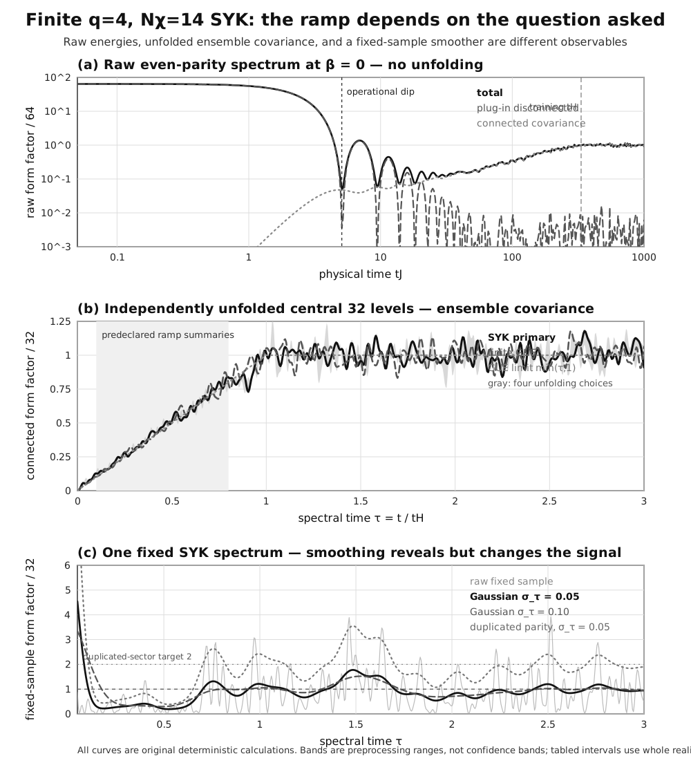
Original deterministic calculation for $q=4$, $N_\chi=14$ SYK at $\beta J=0$. Panel (a) uses all $64$ even-parity levels and physical time $tJ$: solid is the total divided by $64$, long-dashed is the plug-in disconnected estimate, and dotted is the unbiased connected covariance. The marked minimum at $tJ=5.08$ is an operational dip, not $t_{\rm Th}$; the central training spacing gives the local reference $t_HJ=333.10$. Panel (b) uses independently unfolded central $32$-level windows: solid is SYK, long-dashed is matched finite GUE, dotted is $\min(\tau,1)$, and gray is the correlated four-preprocessing range rather than statistical uncertainty. Panel (c) uses one fixed SYK spectrum: Gaussian smoothing widths $\sigma_\tau=0.05$ and $0.10$ reveal different trends, while exact duplication of the symmetry-related parity spectrum raises the target plateau from one to two. Curves are quantitative; jackknife intervals are reported below.

The long-form CSV contains every plotted series and pointwise interval. The structured JSON records the Hamiltonian, seeds, density maps, estimator identities, predeclared bins, sensitivities, runtime, limitations, and scientific-payload fingerprint. The version-controlled checker regenerates the CSV, JSON, and SVG and requires byte-for-byte agreement in --check mode. The materialized scientific payload has SHA-256 fingerprint c491b85547da0671c4ab0ac1f59e20c3521b2a529b75d309cda21b93a8735837; the JSON separately binds the CSV and SVG byte hashes.

Predeclared window summaries

For each interval, the next table gives the mean of $\widehat k_c^U(\tau)$ and a normal-approximation 95% half-width obtained by deleting whole realizations. These are individual interval summaries, not a simultaneous confidence band.

$\tau$ interval	SYK mean $\pm$ 95% half-width	Matched finite GUE mean $\pm$ 95% half-width
$0.05$–$0.10$	$0.0882\pm0.0074$	$0.0775\pm0.0065$
$0.10$–$0.25$	$0.1856\pm0.0096$	$0.1744\pm0.0097$
$0.25$–$0.50$	$0.3841\pm0.0175$	$0.3785\pm0.0164$
$0.50$–$0.80$	$0.6575\pm0.0229$	$0.6659\pm0.0233$
$0.80$–$1.20$	$0.9392\pm0.0234$	$0.9608\pm0.0266$
$1.50$–$3.00$	$1.0019\pm0.0081$	$1.0002\pm0.0082$

The contrasts make the inference boundary clearer.

$\tau$ interval	SYK minus matched GUE	Individual 95% interval
$0.05$–$0.10$	$0.0106$	$[0.0008,0.0204]$
$0.10$–$0.25$	$0.0112$	$[-0.0024,0.0248]$
$0.25$–$0.50$	$0.0056$	$[-0.0184,0.0296]$
$0.50$–$0.80$	$-0.0084$	$[-0.0410,0.0242]$
$0.80$–$1.20$	$-0.0216$	$[-0.0570,0.0138]$
$1.50$–$3.00$	$0.0017$	$[-0.0098,0.0132]$

The earliest bin resolves a small positive difference at this individual-interval level, consistent with early-time finite-window contamination. Every predeclared bin from $\tau=0.10$ onward includes zero. This is not an equivalence test, a multiple-comparison-adjusted statement, or evidence that the complete distributions agree. It says only that this calculation does not resolve a bin-mean difference there. The plateau is consistent with the nondegenerate unit target in both ensembles.

The controls determine the strongest surviving claim

The benchmark changes one analysis choice at a time and records the result rather than treating “reasonable choices” as an undefined robustness test.

Remove the ensemble average. For one fixed spectrum, the mean of $\lvert A_1\rvert^2/32$ over the correlated grid $1.5\le\tau<3$ is $0.9566$, but its coefficient of variation is $0.789$. Gaussian smoothing with $\sigma_\tau=0.025$, $0.05$, and $0.10$ gives plateau-window means $0.9600$, $0.9650$, and $0.9639$. The fitted trend changes sharply with smoothing width and fitting interval. Smoothing makes a trend visible by changing the observable; it supplies neither independent samples nor a disorder-connected covariance Cotler et al. 2017, § 8.

Duplicate the symmetry-related parity block. At $N_\chi\bmod8=6$, the opposite-parity spectrum is an exact symmetry-related copy, not an independent GUE draw. If every level is included twice, the normalized fixed-sample curve is multiplied by two at every $\tau$ and the plateau target becomes two. The resulting curve cannot be compared with the resolved one-block GUE benchmark.

Change the preprocessing and energy-window width. Crossing rank-knot strides $4$ and $8$ with ensemble-density-only and affine-center/interquartile-width preprocessing changes the root-mean-square SYK–GUE curve difference over $0.10\le\tau<3$ only from $0.0745$ to $0.0830$. That small span does not turn the four correlated choices into four replications. The checker separately retains nested central windows of $16$, $24$, and $32$ levels, processes the matched GUE spectra identically, and records each contrast. These are bulk-window-width sensitivities; they do not license an edge-universality claim.

Retained central levels	Curve RMS difference, $0.10\le\tau<3$	Plateau contrast with individual 95% interval
$16$	$0.07908$	$-0.00192$; $[-0.01810,0.01426]$
$24$	$0.07349$	$0.00312$; $[-0.00985,0.01608]$
$32$	$0.07633$	$0.00171$; $[-0.00983,0.01325]$

Move the fitted time interval. With the primary preprocessing, the SYK ramp-slope estimates over $0.10$–$0.40$, $0.20$–$0.60$, and $0.30$–$0.80$ are $0.993$, $0.975$, and $1.008$, with individual 95% intervals $[0.863,1.123]$, $[0.860,1.091]$, and $[0.889,1.127]$. Their jackknife uncertainties delete whole realizations rather than fitting independent errors to the correlated $\tau$ grid. The numerical stability supports a positive finite-size rise over the tested intervals, but one size cannot identify a growing Thouless window.

Keep physical time distinct. The raw calculation gives a central-spacing reference $t_HJ=333.10$ and an operational dip at $tJ=5.08$. The latter is only the minimum of the total raw curve on a predeclared search interval. Calling it $t_{\rm Th}$ would confuse the density-dependent dip with the onset of local RMT behavior; the latter needs a scale-dependent, preferably multi-size comparison Jia and Verbaarschot 2020, § 7.

The strongest surviving claim is therefore:

For $q=4$, $N_\chi=14$ SYK in one resolved even-parity block, the independently unfolded connected form factor of the declared central window has a positive rise and a unit-scale plateau that are descriptively close to an identically processed finite dimension-$64$ GUE ensemble over the tested bins. The conclusion is restricted to this size, ensemble, symmetry block, unfolding family, energy windows, first form-factor moment, and time intervals.

The calculation does not establish a large-$N_\chi$ limit, an expanding universality window, a precise Thouless time, higher form-factor moments, edge universality, sample-specific late-time phases, microscopic unitarity, or a unique JT/SYK duality. A linear mean ramp can coexist with finite-size, edge, sparse-model, or higher-moment departures from dense RMT Legramandi and Talwar 2025, §§ 1, 3.4, and 5.

The JT double trumpet supplies an ensemble ramp

JT gravity makes the ensemble interpretation unusually concrete. In the conventions of Saad, Shenker, and Stanford, the genus-zero double-trumpet contribution is

$$Z_{0,2}(\beta_1,\beta_2) =\frac{\sqrt{\beta_1\beta_2}} {2\pi(\beta_1+\beta_2)}.$$

Analytically continuing $\beta_1=\beta+it$ and $\beta_2=\beta-it$ gives

$$Z_{0,2}(\beta+it,\beta-it) =\frac{\sqrt{\beta^2+t^2}}{4\pi\beta} \sim\frac{\lvert t\rvert}{4\pi\beta} \qquad (\lvert t\rvert\gg\beta).$$

This is the leading connected ensemble ramp Saad, Shenker, and Stanford 2019, § 3.4.1, Eqs. (137)–(139). A chosen nonperturbative matrix-integral completion supplies an ensemble plateau, but the completion is not unique; the perturbative JT data do not select the sample-specific phases of one fixed Hamiltonian Saad, Shenker, and Stanford 2019, §§ 5 and 6.2. Variants with time-reversal symmetry, unorientable surfaces, or additional topological weights map to different random-matrix classes rather than to one universal GUE answer Stanford and Witten 2020, § 2.2.

The double trumpet and the finite-SYK calculation therefore share a class-resolved two-level correlation mechanism under an average. Neither a ramp nor a plateau by itself turns that averaged mechanism into a unique microscopic boundary Hamiltonian. The fixed-theory, factorization, and nonunique-completion questions are treated next in Non-Unique JT Matrix-Integral Completion.

Common pitfalls

One overbar can stand for every average. Disorder averaging, time smoothing, and energy-window averaging act on different objects and can produce different connected subtractions. Name the operation in every formula and caption.

A visible ramp proves chaos. A density transform, a filter, or selected smoothing can imitate part of the shape. A universality claim needs a class-resolved quantitative comparator, uncertainty across independent realizations, and controls chosen before inspecting the curve.

The dip is the Thouless time. The dip is where the falling and rising contributions happen to cross. The Thouless time concerns the onset of RMT correlations and must be defined by a diagnostic and tolerance, ideally across several sizes.

One realization has a disorder-connected form factor. It has $\lvert Z_1\rvert^2$ or $\lvert A_1\rvert^2$. A time smoother can reveal a trend, but it does not manufacture the ensemble covariance $\langle\lvert A\rvert^2\rangle-\lvert\langle A\rangle\rvert^2$.

The infinite GUE triangle is always the fairest comparator. A finite hard window rounds the ideal corner. Process a finite reference ensemble through the identical window, unfolding, normalization, and sample count before interpreting deviations from the large-matrix curve.

The plateau fixes a unique JT/SYK dual. A plateau records discreteness and degeneracy under a declared average. It does not select a unique nonperturbative JT completion or recover the phases and recurrences of one microscopic Hamiltonian.

Exercises

1. Annealed and quenched plateaus

Derive the nondegenerate late-time plateaus of $g_{\rm ann}$ and $g_{\rm q}$. Then replace each distinct energy by a multiplet of degeneracy $d_a$.

Solution

At late time, nondegenerate off-diagonal phases average to zero, leaving

$$\left\lvert Z_j(\beta+it)\right\rvert^2 \longrightarrow \sum_n e^{-2\beta E_{jn}}=Z_j(2\beta).$$

Substitution before or after the ensemble average gives

$$g_{\rm ann}^{\rm plat} =\frac{\langle Z_j(2\beta)\rangle_j} {\langle Z_j(\beta)\rangle_j^2}, \qquad g_{\rm q}^{\rm plat} =\left\langle\frac{Z_j(2\beta)}{Z_j(\beta)^2}\right\rangle_j.$$

For a multiplet, all $d_a^2$ ordered pairs within that exact energy have zero phase difference, so $Z_j(2\beta)$ in the numerator becomes $\sum_a d_a^2e^{-2\beta\varepsilon_{ja}}$.

2. Fourier transform of the GUE sine kernel

Using the fact that the Fourier transform of $(\sin\pi s/\pi s)^2$ is $\max(1-\lvert\tau\rvert,0)$ in the convention $e^{-2\pi i\tau s}$, derive the connected GUE form factor.

Solution

The self-correlation $\delta(s)$ transforms to one. Subtracting the triangular transform gives

$$k_{\rm GUE}(\tau) =1-\max(1-\lvert\tau\rvert,0) =\begin{cases} \lvert\tau\rvert,&\lvert\tau\rvert\le1,\\ 1,&\lvert\tau\rvert\ge1. \end{cases}$$

Omitting the self-correlation would omit the plateau and change the meaning of the plotted object.

3. The finite-sample decomposition

Prove the identity between $\widehat{\mathcal K}_{\rm tot}$, the plug-in disconnected estimator, and the unbiased connected covariance.

Solution

For complex numbers $Z_j$,

$$\sum_{j=1}^R\left\lvert Z_j-\overline Z\right\rvert^2 =\sum_{j=1}^R\left\lvert Z_j\right\rvert^2 -R\left\lvert\overline Z\right\rvert^2.$$

Divide by $RD$. The first term becomes $\widehat{\mathcal K}_{\rm tot}$, the second becomes $\widehat{\mathcal K}_{\rm disc}^{\rm plug}$, and the left side is $(R-1)\widehat{\mathcal K}_{\rm conn}^{U}/R$. Rearranging gives the displayed identity. The factor $(R-1)/R$ is essential because the connected estimator is unbiased while the disconnected estimator is a plug-in square of the sample mean.

4. An unresolved parity copy

Suppose a resolved block has amplitude $A(\tau)$ and plateau-normalized form factor $\lvert A\rvert^2/M$. What happens if an exactly isospectral partner block is concatenated and the normalization uses the new total of $2M$ levels?

Solution

The concatenated amplitude is $A_{\rm dup}=2A$. Hence

$$\frac{\left\lvert A_{\rm dup}\right\rvert^2}{2M} =\frac{4\lvert A\rvert^2}{2M} =2\frac{\lvert A\rvert^2}{M}.$$

The entire curve, including its plateau, doubles. The correct remedy is to resolve the symmetry-related blocks before comparing with a one-block GUE ensemble, not to reinterpret the doubled plateau as a new universality class.

5. The double-trumpet claim boundary

Continue the double-trumpet expression to $\beta\pm it$, derive its late-time growth, and explain why this does not derive the plateau of one fixed Hamiltonian.

Solution

The product of the two square-root arguments is $\beta^2+t^2$, while their sum is $2\beta$. Therefore

$$Z_{0,2}(\beta+it,\beta-it) =\frac{\sqrt{\beta^2+t^2}}{4\pi\beta} \sim\frac{\lvert t\rvert}{4\pi\beta}.$$

This genus-zero connected contribution gives an ensemble ramp. A plateau requires nonperturbative spectral discreteness in a chosen completion. The perturbative saddle does not specify the individual energy gaps and phases that control the quasiperiodic signal and recurrences of one fixed Hamiltonian, nor does it select a unique completion.

The chapter overview contains the structure diagram and validity and failure diagram. They are embedded there once so that their shared chapter-level context is not repeated on every article.

For the chapter-wide comparison of assumptions, counterevidence, falsifiers, and claim ceilings, see the claim-domain table.

References

• Cotler, Jordan S., Guy Gur-Ari, Masanori Hanada, Joseph Polchinski, Phil Saad, Stephen H. Shenker, Douglas Stanford, Alexandre Streicher, and Masaki Tezuka. “Black Holes and Random Matrices.” Journal of High Energy Physics 2017, 5 (2017): 118; erratum 2018, 9 (2018): 2. DOI. Open PDF.
• Jia, Yiyang, and Jacobus J. M. Verbaarschot. “Spectral Fluctuations in the Sachdev–Ye–Kitaev Model.” Journal of High Energy Physics 2020, 7 (2020): 193. DOI. Open PDF.
• Legramandi, Andrea, and Neil Talwar. “The Moments of the Spectral Form Factor in SYK.” Journal of High Energy Physics 2025, 8 (2025): 108. DOI. Open PDF.
• OpenAI Codex for QFT.org. “Finite-SYK Spectral-Form-Factor Benchmark and Analysis Controls.” Python source, CSV, JSON, and SVG, validated 29 August 2026. Source SHA-256 eef80283b318edc0bb30567338c63bf898881c7c367f105677c6bab8f256adc5. Python source on GitHub.
• Prange, R. E. “The Spectral Form Factor Is Not Self-Averaging.” Physical Review Letters 78, no. 12 (1997): 2280–2283. DOI. Open preprint.
• Saad, Phil, Stephen H. Shenker, and Douglas Stanford. “JT Gravity as a Matrix Integral.” arXiv:1903.11115 [hep-th] (2019). Preprint. Open PDF.
• Stanford, Douglas, and Edward Witten. “JT Gravity and the Ensembles of Random Matrix Theory.” Advances in Theoretical and Mathematical Physics 24, no. 6 (2020): 1475–1680. DOI. Open PDF.