Gauge Fields in Two Dimensions

The previous two pages studied one-dimensional fermions from the many-body side. We found that the Fermi surface collapses to two Fermi points, that low-energy fields split into right- and left-movers, and that logarithms appear because the kinematics are effectively two-dimensional: one time direction and one space direction.

We now reorganize the same physics in the language of relativistic two-dimensional field theory. The great simplification is that a massless fermion in $1+1$ dimensions separates into two chiral components. Each component is governed by a first-order operator in one light-cone direction. As a result, the fermion Green function in an arbitrary Abelian background gauge field can be written almost exactly by inspection. This is the technical seed of the Schwinger model, the Thirring model, bosonization, and many of the two-dimensional examples that follow.

There is another simplification, just as important: a gauge field in $1+1$ dimensions has no transverse photon polarization. This does not mean that gauge fields are irrelevant. It means that their dynamics are mostly constraint, topology, holonomy, and vacuum polarization rather than propagating waves. Two dimensions are small enough to solve many things and still large enough for anomalies, confinement, screening, and nontrivial operator dimensions to show up. Tiny arena, dramatic cast.

Required background. Fermi-surface instabilities and one-dimensional fermions supplies the right-/left-moving decomposition and the logarithms that become anomalous powers below. Helpful background. Current correlators and polarization tensors supplies the transverse response kernel used for the fermion determinant, while Ward identities and chiral symmetries supplies the gauge-covariance logic. Three related objects remain distinct throughout: the fixed-background propagator $G(x,y;A)$ is gauge covariant and carries endpoint phases; the closed-loop determinant $e^{-W[A]}$ controls vacuum polarization; and a gauge-invariant observable is neutral or includes a Wilson-line dressing. In a dynamical gauge theory, a charged propagator may be useful in a chosen gauge, but physical operators must respect the gauge constraint. The auxiliary vector used for a current interaction below does not introduce that same gauge redundancy.

Gauge fields without transverse photons

Light-cone conventions. On this page we use real-time light-cone coordinates

$$x^+=x^0+x^1, \qquad x^-=x^0-x^1,$$

with

$$\partial_+={1\over2}(\partial_0+\partial_1), \qquad \partial_-={1\over2}(\partial_0-\partial_1).$$

The line element is

$$ds^2=dx^+dx^-.$$

The gauge field one-form is written as

$$A=A_+dx^+ + A_-dx^-,$$

These are coordinate one-form components. They are related to the full Cartesian sums used in lessons 19 and 20 by

$$A_+={A_0+A_1\over2}={\widehat A_+\over2}, \qquad A_-={A_0-A_1\over2}={\widehat A_-\over2}.$$

The gauge transformation is

$$A_\pm\mapsto A_\pm+\partial_\pm\theta.$$

For a unit-charge field, the covariant derivatives are

$$D_\pm=\partial_\pm-iA_\pm, \qquad \psi\mapsto e^{+i\theta}\psi.$$

Following lessons 19 and 20, the subscripts on the chiral fields are propagation labels rather than $\gamma^5$ eigenvalues: $\psi_+=P_-\psi$ is acted on by $D_-$, while $\psi_-=P_+\psi$ is acted on by $D_+$.

We order the light-cone measure as $dx^+dx^-$ and use its positive coordinate density. Since the absolute Jacobian is $dx^0dx^1=\frac12dx^+dx^-$, the factor $2$ in each Cartesian-measure chiral kinetic term cancels the Jacobian. Likewise $\widehat A_\pm=2A_\pm$ converts the Cartesian source coupling to the unit coefficients displayed below. To keep the inverse equations unambiguous, define

$$\delta^{(2)}_{\mathrm{LC}}(x-y) =\delta(x^+-y^+)\delta(x^--y^-),$$

the delta function normalized with the measure $dx^+dx^-$. The Cartesian delta function normalized with $dx^0dx^1$ is $2\delta^{(2)}_{\mathrm{LC}}$. With the propagation labels above, the light-cone Green functions satisfy $D_+G_-=D_-G_+=\delta^{(2)}_{\mathrm{LC}}$.

In four spacetime dimensions, a massless gauge boson has two physical transverse polarizations. In $1+1$ dimensions there is no transverse direction. The gauge potential has two components, $A_0$ and $A_1$; gauge redundancy removes one combination, and Gauss’ law removes the other as an independent local oscillator. The gauge-invariant field strength has only one component,

$$F_{01}=\partial_0A_1-\partial_1A_0.$$

It is an electric field, not a wave with transverse polarizations.

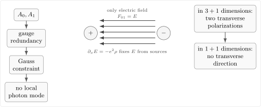
In $1+1$ dimensions there is no transverse direction for a photon. The electric field $F_{01}$ is still physical, but it is fixed by constraints and sources rather than by an independent transverse wave mode.

This statement is clearest in temporal gauge, $A_0=0$. The Maxwell action is

$$S_M={1\over2e^2}\int d^2x\,E^2, \qquad E=\partial_0A_1.$$

The equation obtained by varying $A_0$ before imposing the gauge is Gauss’ law,

$$\partial_1E=-e^2\rho.$$

For external static charges, Gauss’ law determines $E$ algebraically from the charge distribution. Between a charge and an anticharge, the electric field is constant; the energy grows linearly with separation. This is the elementary reason why two-dimensional electrodynamics is a useful toy model for confinement, even though the detailed story depends strongly on whether light dynamical fermions are present.

In the absence of matter, the equation of motion

$$\partial_\mu F^{\mu\nu}=0$$

says in two dimensions that $F_{01}$ is constant locally. There is no local photon Hilbert space. But once fermions are integrated out, the gauge field can acquire a nonlocal effective action and, in the Schwinger model, a gauge-invariant mass scale. That will be one of the next lessons.

Massless fermions and chiral splitting

A massless Dirac fermion in two dimensions decomposes into two independent chiral components. Retaining the propagation-label convention declared above, write

$$\psi=\psi_+ + \psi_-, \qquad \psi_+=P_-\psi, \qquad \psi_-=P_+\psi.$$

The massless action separates exactly into two first-order pieces in the ordered light-cone measure:

$$S_0=i\int dx^+dx^-\, \left( \psi_-^\dagger\partial_+\psi_-+ \psi_+^\dagger\partial_-\psi_+ \right).$$

Thus the free equations are

$$\partial_+\psi_-=0, \qquad \partial_-\psi_+=0.$$

The field $\psi_-$ depends only on $x^-$, while $\psi_+$ depends only on $x^+$. In ordinary coordinates these are right- and left-moving fields. Coupling to a background Abelian gauge field gives

$$S[A]=i\int dx^+dx^-\, \left[ \psi_-^\dagger(\partial_+ - iA_+)\psi_- + \psi_+^\dagger(\partial_- - iA_-)\psi_+ \right].$$

The two chiralities couple to different light-cone components of the gauge field. This is why two-dimensional fermion problems often reduce to one-dimensional inverse operators.

For the $\psi_-$ component, define the background Green function by

$$(\partial_+ - iA_+(x))G_-(x,y;A)=\delta^{(2)}_{\mathrm{LC}}(x-y).$$

The $\psi_+$ equation is obtained by exchanging $+\leftrightarrow-$:

$$(\partial_- - iA_-(x))G_+(x,y;A)=\delta^{(2)}_{\mathrm{LC}}(x-y).$$

Because each equation contains only one derivative, the background field enters as a phase or Wilson line.

The free chiral propagator

The free inverse of $\partial_+$ is not simply $1/x^+$. The operator $\partial_+$ differentiates along $x^+$, but the chiral singularity sits at fixed $x^-$. With ordinary time ordering, the useful distribution is

$$\boxed{ G_-^{(0)}(x-y)= {1\over2\pi i}\, {1\over x^- - y^- - i0\,\operatorname{sgn}(x^+ - y^+)}. }$$

It satisfies

$$\partial_{x^+}G_-^{(0)}(x-y)=\delta^{(2)}_{\mathrm{LC}}(x-y).$$

The reason the $i0$ prescription involves $\operatorname{sgn}(x^+-y^+)$ is subtle the first time one sees it, but perfectly logical. The pole is at $x^-=y^-$. On that singular support,

$$x^0-y^0={1\over2}(x^+-y^+),$$

so ordinary time ordering is equivalent to ordering in $x^+$ at the pole. The discontinuity of the pole as $x^+-y^+$ crosses zero is exactly what produces the two-dimensional delta function.

Similarly,

$$\boxed{ G_+^{(0)}(x-y)= {1\over2\pi i}\, {1\over x^+ - y^+ - i0\,\operatorname{sgn}(x^- - y^-)} }$$

satisfies

$$\partial_{x^-}G_+^{(0)}(x-y)=\delta^{(2)}_{\mathrm{LC}}(x-y).$$

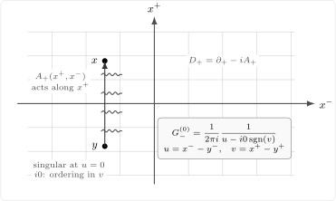
For the $\psi_-$ chirality, the operator is $D_+=\partial_+ - iA_+$. The free propagator is singular on $x^-=y^-$, and the integrating factor accumulates $A_+$ along each fixed-$x^-$ ray. A general bilocal Green function still requires both endpoint factors.

The propagator formula also gives the equal-time canonical anticommutator. The difference between the two time orderings is

$${1\over u-i0}-{1\over u+i0}=2\pi i\delta(u),$$

so the jump of $G_-^{(0)}$ across $x^0=y^0$ reproduces the delta function in the spatial coordinate.

Euclidean bridge to complex coordinates

The real-time light-cone formulas have a Euclidean version that will be used heavily in the bosonization page. Set $x^2=\tau$ after Wick rotation and introduce

$$z=x^1+ix^2, \qquad \bar z=x^1-ix^2,$$

with

$$\partial_z={1\over2}(\partial_1-i\partial_2), \qquad \partial_{\bar z}={1\over2}(\partial_1+i\partial_2).$$

To keep the normalization explicit, define the canonical Euclidean chiral fields by

$$S_E=2\int d^2x\, \left(\psi_R^\dagger\partial_{\bar z}\psi_R +\psi_L^\dagger\partial_z\psi_L\right).$$

The conjugate Grassmann fields are independently continued along with the action; an overall real-time phase is not removed merely by renaming the coordinates. Since $\partial_{\bar z}(1/z)=\pi\delta^{(2)}_E(z)$, inversion of the kinetic operator gives

$$\langle\psi_R(z)\psi_R^\dagger(w)\rangle ={1\over2\pi(z-w)}, \qquad \langle\psi_L(\bar z)\psi_L^\dagger(\bar w)\rangle ={1\over2\pi(\bar z-\bar w)}.$$

Conformal-field-theory calculations often use the rescaled fields $\Psi_{R,L}=\sqrt{2\pi}\,\psi_{R,L}$. Their action has coefficient $1/\pi$ in place of $2$, and their propagators are

$$\langle \Psi_R(z)\Psi_R^\dagger(w)\rangle={1\over z-w},$$

and

$$\langle \Psi_L(\bar z)\Psi_L^\dagger(\bar w)\rangle={1\over \bar z-\bar w}.$$

The kinetic inverse and this unit-OPE choice can be checked directly in Di Francesco, Mathieu, and Sénéchal 1997, §5.3.2, pp.129–130, Eqs.(5.87)–(5.93), and §6.4.1, p.168, Eqs.(6.96)–(6.97). Their real-fermion kinetic normalization is called $g$; it is unrelated to the current-interaction coupling below. Combining two real fermions gives the complex fields used here.

The currents must be rescaled with the fields. For example,

$$J_R=:\!\Psi_R^\dagger\Psi_R\!: =2\pi j_R, \qquad j_R=:\!\psi_R^\dagger\psi_R\!:.$$

Thus a physical source couples to $J_R/(2\pi)$, and two current insertions supply the compensating factor $(2\pi)^{-2}$. The physical polarization kernel is unchanged. We return to canonical $\psi$ and $j_\mu=\bar\psi\gamma_\mu\psi$ in the determinant and auxiliary-field sections. The Abelian bosonization dictionary likewise keeps the fermion’s UV normalization and physical current explicit.

The distributional $i0$ prescriptions above are the Lorentzian ancestors of these holomorphic singularities. With a fixed field normalization, determinants of chiral propagators become Cauchy determinants, which free-boson vertex operators can reproduce.

Exact Abelian Green functions in a background field

Now suppose first that the background is Abelian. Locally, for any fixed $x^-$, we can write

$$A_+(x^+,x^-)=\partial_+\alpha(x^+,x^-),$$

where, more precisely,

$$\alpha(x^+,x^-) =\alpha_0(x^-)+\int_{x_0^+}^{x^+}ds\,A_+(s,x^-)$$

for some reference point $x_0^+$ and boundary datum $\alpha_0(x^-)$. This is not a gauge-fixing assumption and does not imply that the full field strength vanishes. It is only the statement that a one-dimensional connection along the $x^+$ direction can be integrated. The freedom in $\alpha_0$ is part of the boundary prescription for the first-order inverse.

With $D_+=\partial_+ - iA_+$, an exact Green inverse with the conjugated free boundary prescription is

$$\boxed{ G_-(x,y;A)= e^{+i\alpha(x)}G_-^{(0)}(x-y)e^{-i\alpha(y)}. }$$

Indeed,

$$(\partial_+ - i\partial_+\alpha) \left(e^{+i\alpha(x)}G_-^{(0)}(x-y)e^{-i\alpha(y)}\right) =e^{+i\alpha(x)}\partial_+G_-^{(0)}(x-y)e^{-i\alpha(y)}.$$

Using $\partial_+G_-^{(0)}=\delta^{(2)}_{\mathrm{LC}}$, the phase factors cancel at $x=y$, so

$$D_+G_-(x,y;A)=\delta^{(2)}_{\mathrm{LC}}(x-y).$$

This equation alone does not select a unique vacuum inverse. At fixed $A$, replacing $\alpha$ by $\alpha+f(x^-)$ changes the displayed kernel to

$$G_-^{\,f}(x,y;A) =e^{if(x^-)}G_-(x,y;A)e^{-if(y^-)}.$$

Both kernels have the same delta-function source, so $D_+^x(G_-^{\,f}-G_-)=0$. For $A=0$ and $f(x^-)=a x^-$, their nonzero difference is $(e^{ia(x^--y^-)}-1)G_-^{(0)}(x-y)$, a homogeneous solution. Selecting the same physical state requires keeping its boundary condition fixed, or transforming the boundary kernel to compensate; arbitrary primitive choices are not interchangeable Feynman prescriptions.

The same construction for the other chirality gives

$$A_- = \partial_-\beta,$$

and

$$\boxed{ G_+(x,y;A)= e^{+i\beta(x)}G_+^{(0)}(x-y)e^{-i\beta(y)}. }$$

Under a gauge transformation, choose the boundary datum to transform as $\alpha_0(x^-)\mapsto\alpha_0(x^-)+\theta(x_0^+,x^-)$. Then $\alpha\mapsto\alpha+\theta$ and

$$G_-(x,y;A+\partial\theta) =e^{+i\theta(x)}G_-(x,y;A)e^{-i\theta(y)}.$$

The essential point is that the background field changes a chiral propagator by endpoint phases. This is the two-dimensional ancestor of several statements that will appear later: Wilson-line dressing, anomalous power laws, bosonization, and the exact solvability of the Schwinger model.

Gauge decomposition and field strength

Since $A_+$ and $A_-$ can each be integrated along their own light-cone direction, write

$$A_+=\partial_+\alpha, \qquad A_-=\partial_-\beta.$$

The field strength is

$$F_{+-}=\partial_+A_- - \partial_-A_+ =\partial_+\partial_-(\beta-\alpha).$$

For compatible choices of the primitives, define their difference

$$\varphi=\beta-\alpha.$$

Under a gauge transformation,

$$A_\pm\mapsto A_\pm+\partial_\pm\theta,$$

we have

$$\alpha\mapsto\alpha+\theta, \qquad \beta\mapsto\beta+\theta,$$

and hence

$$\varphi\mapsto\varphi.$$

There is also an independent freedom at fixed $A$:

$$\alpha\mapsto\alpha+f(x^-), \qquad \beta\mapsto\beta+g(x^+), \qquad \varphi\mapsto\varphi+g(x^+)-f(x^-).$$

The mixed derivative removes these one-variable terms. Consequently $\varphi$ is invariant under the common gauge shift, but it is not a unique functional of $A$ until the primitive boundary data have been fixed. The curvature $F_{+-}$ is independent of both choices. The next diagram separates these two operations.

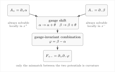
The electric field is determined by a mixed derivative of the primitive difference. Common gauge shifts cancel in that difference; the independent one-variable primitive shifts disappear after differentiation. A nonzero difference can still describe a zero field. This schematic local construction fixes boundary and global data separately.

On a contractible rectangular patch, $F_{+-}=0$ implies $\partial_+\partial_-\varphi=0$, hence $\varphi=u(x^+)+v(x^-)$. Choosing $f=v$ and $g=-u$ makes the new primitives equal, so the field is locally pure gauge. Conversely, equal primitives give $F_{+-}=0$. The correct criterion is zero curvature, not zero difference for every primitive choice: $A_\pm=0$, $\alpha=\sin x^-$, and $\beta=0$ give $\varphi=-\sin x^-\neq0$ with zero field strength.

On a space with nontrivial topology, such as a spatial circle or a thermal cylinder, there can also be zero modes and holonomies that are not captured by a single-valued local $\alpha$ or $\beta$. Those global variables are important in precise treatments, but the local formulas above are the workhorse for perturbative and operator calculations.

Fermion determinant and open-line propagator

There are two different objects that one must not confuse. The first is the open-line Green function in a fixed background,

$$G(x,y;A)=\langle x|(\gamma^\mu D_\mu)^{-1}|y\rangle.$$

The second is the fermion determinant, obtained by integrating out closed fermion loops:

$$e^{-W_E[A]} =\int \mathcal D\bar\psi\mathcal D\psi\, \exp\left[-\int d^2x\,\bar\psi\gamma^\mu D_\mu\psi\right] =\det(\gamma^\mu D_\mu).$$

Equivalently,

$$W_E[A]=-\operatorname{Tr}\log(\gamma^\mu D_\mu).$$

In a theory where the gauge field is also integrated over, the full fermion two-point function has the schematic form

$$\boxed{ \langle \psi(x)\bar\psi(y)\rangle ={1\over Z}\int \mathcal D A\, e^{-S_{g,E}[A]-W_E[A]}G(x,y;A). }$$

Here

$$Z=\int \mathcal D A\,e^{-S_{g,E}[A]-W_E[A]}.$$

The open propagator has an expansion in insertions of the background field,

$$G[A] =G_0+G_0(i\gamma^\mu A_\mu)G_0 +G_0(i\gamma^\mu A_\mu)G_0(i\gamma^\mu A_\mu)G_0+\cdots,$$

while $W[A]$ is made of closed fermion loops.

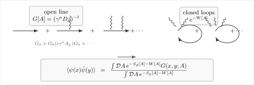
For fixed $A$, the open line gives $G[A]=(\gamma^\mu D_\mu)^{-1}$. Integrating out fermions also produces closed loops collected into $W[A]$. The full correlator averages the open line with the determinant included in the weight.

This distinction matters. If one averages $G(x,y;A)$ over $A$ but forgets $W[A]$, one has neglected vacuum polarization. That omission can define a controlled quenched approximation, but it is not the original dynamical-fermion theory. In two dimensions it misses precisely the closed-loop response responsible for the anomaly-related infrared physics.

For a massless unit-charge Dirac fermion on the Euclidean plane, preserving vector gauge invariance gives the universal nonlocal part of the Abelian determinant,

$$W_E[A] ={1\over2\pi}\int d^2x\, A_\mu \left(\delta_{\mu\nu}-{\partial_\mu\partial_\nu\over\partial^2}\right) A_\nu.$$

Equivalently,

$$W_E[A] ={1\over2\pi}\int d^2x\, F_{12}{1\over-\partial^2}F_{12}.$$

The coefficient is the unit-current transverse kernel derived in Current correlators and polarization tensors, with its stated Euclidean continuation. For an explicit two-insertion calculation, see Morais and Mota 2009, §III, p.4, Eqs.(12)–(15), PDF. Their connection couples as $-eA_\mu j^\mu$; reversing the sign at both insertions leaves the positive $e^2/\pi$ coefficient unchanged. Here the charge is absorbed into $A$, giving $1/\pi$. No reversal of the current convention is needed.

This formula is finite and nonlocal. A renormalization prescription may separately add local gauge-invariant counterterms, such as a Maxwell term; it may not add an arbitrary longitudinal mass term while claiming to preserve the vector Ward identity. On a compact surface, flux sectors, harmonic gauge fields, spin structures, and fermion zero modes also contribute global factors not contained in this plane-wave kernel.

The connection to the primitive construction becomes especially transparent in the Euclidean Hodge decomposition. For the following rewrite, take smooth $\lambda,\chi$ decreasing rapidly with their derivatives on the plane, and fix their constant modes to zero. More general boundary conditions are allowed only when they fix the harmonic ambiguity and give the same vanishing boundary terms. Write

$$A_\mu=\partial_\mu\lambda+\epsilon_{\mu\nu}\partial_\nu\chi, \qquad \epsilon_{12}=+1.$$

With that prescription the transverse projector removes $\partial_\mu\lambda$, while

$$F_{12}=-\partial^2\chi.$$

Choose $\chi=(-\partial^2)^{-1}F_{12}$ in the specified inverse domain. After an integration by parts with zero boundary contribution,

$$\boxed{ W_E[A]={1\over2\pi}\int d^2x\,(\partial_\mu\chi)^2. }$$

Thus the determinant depends on curvature through this fixed transverse representative. Simple connectedness alone is insufficient: on a unit square, $\chi=x^1$ and $\lambda=x^2$ give $A_\mu=0$ but $\int(\partial\chi)^2=1$. The boundary term omitted in the displayed rewrite is then nonzero. This is the Euclidean version of the need to fix primitive nullspaces, not an additional contribution to the determinant of a zero field. When the gauge field has its own Maxwell action, the same nonlocal term produces the mass scale of the Schwinger model.

A useful normalization check is the following. In momentum space this same term is

$$W_E[A]={1\over2}\int_p A_\mu(-p)\,{1\over\pi}P^T_{\mu\nu}(p)\,A_\nu(p), \qquad P^T_{\mu\nu}=\delta_{\mu\nu}-{p_\mu p_\nu\over p^2}.$$

When it is added to the Maxwell term $(2e^2)^{-1}\int_p p^2 A^T_\mu(-p)A^T_\mu(p)$, the transverse denominator is $p^2/e^2+1/\pi$. Thus the mass in the next page is $m_\gamma^2=e^2/\pi$, not $2e^2/\pi$. The factor of $1/2$ in the quadratic-action convention is doing real work here.

Auxiliary gauge fields and current interactions

The same background-field method also organizes current-current interactions. Consider the Euclidean Thirring-type interaction

$$\mathcal L_E =\bar\psi\gamma_\mu\partial_\mu\psi +{g\over2}j_\mu j_\mu, \qquad j_\mu=\bar\psi\gamma_\mu\psi.$$

For $g>0$, introduce a real auxiliary vector field. With a finite regulator the identity is the normalized Gaussian characteristic function, applied to each real mode:

$${1\over(2\pi g)^{N/2}}\int_{\mathbb R^N}d^NA\, e^{-A^2/(2g)+iA\cdot j} =e^{-g j^2/2}.$$

Restoring the functional notation gives

$$\exp\left[-{g\over2}\int d^2x\,j_\mu j_\mu\right] \propto \int \mathcal D A_\mu\, \exp\left[-\int d^2x\, \left({1\over2g}A_\mu A_\mu-iA_\mu j_\mu\right)\right].$$

For real mode sources the identity follows by Fourier transformation of the convergent Gaussian; for finite Grassmann currents it holds term by term in their nilpotent expansion. At $g=0$ use the free limit. For $g<0$ the real contour diverges: a continuation would require a specified complex contour, such as $A=iB$ mode by mode, and cannot be described as this positive real Gaussian measure. This restriction on the representation is not a derivation of the complete Thirring model’s allowed coupling range.

The auxiliary action includes $A^2/(2g)$, so it does not impose the gauge redundancy of a dynamical Maxwell theory. Its fermion determinant is nevertheless the same background-covariant determinant. Thus the interacting fermion problem becomes a free fermion in a fluctuating background $A_\mu$, followed by an average over $A_\mu$ with the determinant included. For a chiral component, the background-field answer gives the schematic, consistently continued structure

$$\langle T\psi_-(x)\psi_-^\dagger(y)\rangle =G_-^{(0)}(x-y) \left\langle e^{+i[\alpha(x)-\alpha(y)]}\right\rangle_A.$$

To see how an anomalous power can arise, work first in Euclidean separation $r_E^2=(\Delta x^1)^2+(\Delta\tau)^2$. Suppose a centered real Gaussian endpoint variable $X$ has, at $r_E\gtrsim a$,

$$\langle X^2\rangle =\kappa\log{r_E^2\over a^2}+\text{constant}, \qquad \kappa\geq0,$$

then

$$\left\langle e^{iX}\right\rangle =\exp\left[-{1\over2}\langle X^2\rangle\right] \propto \left({a^2\over r_E^2}\right)^{\kappa/2}.$$

Multiplying a free chiral kernel by this factor gives an anomalous power law. For a time-ordered continuation use the same vacuum prescription as the free chiral kernel and the branch reached from positive $r_E^2$:

$r_E^2\longrightarrow (\Delta x^1)^2-(|\Delta t|-i0)^2.$

Under the stated endpoint-cumulant assumption this gives

$$\langle T\psi_-(x)\psi_-^\dagger(y)\rangle \propto {1\over x^- - y^- - i0\operatorname{sgn}(x^+-y^+)} \left({a^2\over(\Delta x^1)^2-(|\Delta t|-i0)^2}\right)^{\kappa/2}.$$

This calculation illustrates the mechanism; it does not calculate $\kappa(g)$. In an actual Euclidean background problem a chiral primitive can be complex, and its endpoint cumulant, mean, and continuation must be derived with the chosen boundary prescription rather than assumed to be a real variance. A fluctuating gauge or auxiliary field can change the scaling dimension of the fermion itself. In later language, the fermion behaves like an exponential of a free boson.

Abelian and non-Abelian backgrounds

For Abelian backgrounds, a single chiral equation is solved by an ordinary phase. For a non-Abelian background, $A_+$ is matrix-valued. Introduce a group-valued integrating factor $g(x)$ satisfying

$$(\partial_+ - iA_+)g=0.$$

At fixed $x^-$ it can be written as

$$g(x^+,x^-) =\mathcal P\exp\left[+i\int_{x_0^+}^{x^+}ds\,A_+(s,x^-)\right]g_0(x^-),$$

where $g_0(x^-)$ supplies the boundary data. The exact local inverse is then

$$\boxed{ G_-(x,y;A)=g(x)G_-^{(0)}(x-y)g^{-1}(y). }$$

Indeed, $D_+^xg(x)=0$, and on the support of $\partial_+G_-^{(0)}=\delta^{(2)}_{\mathrm{LC}}$ the matrix factors become $g(x)g^{-1}(x)=1$. If a gauge transformation acts as $\psi\mapsto h\psi$, the compatible choice $g\mapsto hg$ gives

$$G_-(x,y;A^h)=h(x)G_-(x,y;A)h^{-1}(y).$$

This is the non-Abelian version of the Abelian endpoint phases. Path ordering is essential because the matrices $A_+(s,x^-)$ at different $s$ need not commute.

The non-Abelian determinant is much richer than the Abelian one. The analogue of $W[A]$ contains the two-dimensional current algebra structure and is closely related to the Wess–Zumino–Witten functional. That is why the innocent-looking replacement

$$\bar\psi\gamma_\mu\psi \quad\longrightarrow\quad \bar\psi\gamma_\mu T^a\psi$$

changes the theory qualitatively. Closed loops now carry group generators, path ordering matters, and the effective action is no longer Gaussian in a single scalar phase.

Boundary data and Wilson-line shorthand

There is a small but consequential geometric point hidden by the usual Wilson-line shorthand. The segment

$$U(x^+,y^+;x^-) =\mathcal P\exp\left[+i\int_{y^+}^{x^+}ds\,A_+(s,x^-)\right].$$

obeys

$$(\partial_+ - iA_+(x))U(x^+,y^+;x^-)=0, \qquad U(y^+,y^+;x^-)=1.$$

But its lower endpoint is $(y^+,x^-)$, not the spacetime point $y=(y^+,y^-)$. Unless $x^-=y^-$, it therefore transforms with $\theta(y^+,x^-)$ rather than $\theta(y)$. The tempting expression

$$U(x^+,y^+;x^-)G_-^{(0)}(x-y)$$

solves the differential equation in its first argument but is not, by itself, the generally gauge-covariant bilocal Green function.

The endpoint-factor formula avoids this mistake. It transports $x$ and $y$ to boundary data on a reference slice and keeps both endpoint transformations:

$$G_-(x,y;A)=e^{+i\alpha(x)}G_-^{(0)}(x-y)e^{-i\alpha(y)}.$$

In the Abelian case, this endpoint phase equals the Wilson line of the given $A$ along the path $y\to(x_0^+,y^-)\to(x_0^+,x^-)\to x$ only if the reference datum satisfies

$${d\alpha_0(u)\over du}=A_-(x_0^+,u).$$

Then the middle segment contributes

$$\int_{y^-}^{x^-}du\,A_-(x_0^+,u) =\alpha_0(x^-)-\alpha_0(y^-),$$

and the three segment integrals add to $\alpha(x)-\alpha(y)$. For arbitrary $\alpha_0$, the middle factor is boundary data and need not be the line integral of that same $A$. The local equation $D_+G=\delta^{(2)}_{\mathrm{LC}}$ does not impose this extra condition or select a state. Retarded, advanced, Feynman, finite-temperature, and finite-volume inverses additionally specify their boundary and state prescriptions.

On a circle or thermal cylinder, this boundary information includes holonomy and zero-mode sectors. The local integrating-factor solution remains correct, but no single-valued $\alpha$ or $g$ captures the entire answer globally.

Summary

Two-dimensional gauge theory is special for two independent reasons. First, the gauge field has no local transverse photon polarization. Its physical content is encoded in the electric field, constraints, holonomies, and the response of matter. Second, massless fermions split into chiral components, and each chiral component couples to only one light-cone component of the gauge field.

The central formula on this page is the exact chiral background propagator

$$G_-(x,y;A)=e^{+i\alpha(x)}G_-^{(0)}(x-y)e^{-i\alpha(y)}, \qquad A_+=\partial_+\alpha,$$

with the analogous formula for $G_+$. This formula turns the problem of fermions in a fluctuating gauge or auxiliary field into the problem of averaging endpoint phases. In two dimensions such averages often produce logarithms, and exponentiated logarithms become anomalous powers. That is the bridge from Fermi-point logarithms to bosonization and exactly solvable models.

Common pitfalls

Confusing a directional primitive with a pure gauge. The statement $A_+=\partial_+\alpha$ is local and one-dimensional. It does not mean that the full gauge field is pure gauge. Curvature is the mixed derivative of $\beta-\alpha$; a nonzero primitive difference can still give zero curvature.

Differentiating the wrong coordinate. The free chiral propagator for $\partial_+$ is singular in $x^-$, not in $x^+$. The derivative with respect to $x^+$ acts on the time-ordering prescription. This is a classic source of confused signs and missing delta functions.

Replacing endpoint phases by the wrong Wilson segment. A light-cone segment at fixed $x^-$ ends at $(y^+,x^-)$, not at a general point $(y^+,y^-)$. Use the two endpoint factors, or specify the reference-slice connector and boundary condition explicitly.

Equating the determinant with the open propagator. The determinant $W[A]$ is not the same object as the open propagator $G[A]$. Dropping $W[A]$ means dropping closed fermion loops. In two dimensions those loops can change the infrared physics completely.

Treating the absence of transverse photons as the absence of gauge physics. A two-dimensional gauge field has no local photon polarization, but it can mediate a linear Coulomb potential, carry holonomies, impose constraints, and acquire a gauge-invariant mass scale through matter polarization.

Exercises

Exercise 1: Verify the light-cone contact term

Verify the distribution identity

$$\partial_+\left[{1\over2\pi i}\,{1\over x^- - i0\operatorname{sgn}x^+}\right] =\delta(x^+)\delta(x^-).$$

Solution

For $x^+\neq0$, the sign is constant and the expression has no explicit smooth dependence on $x^+$, so the derivative vanishes away from $x^+=0$. The whole derivative is a contact term at $x^+=0$.

Across $x^+=0$, the denominator changes from $x^-+i0$ to $x^- - i0$. More precisely,

$$\partial_+{1\over x^- - i0\operatorname{sgn}x^+} =\delta(x^+)\left({1\over x^- - i0}-{1\over x^- + i0}\right).$$

Using

$${1\over u-i0}-{1\over u+i0}=2\pi i\delta(u),$$

we obtain

$$\partial_+{1\over x^- - i0\operatorname{sgn}x^+} =2\pi i\delta(x^+)\delta(x^-).$$

Multiplying by $1/(2\pi i)$ gives the desired result.

Exercise 2: Verify the exact Abelian background propagator

Let $D_+=\partial_+ - iA_+$ and suppose $A_+=\partial_+\alpha$. Show that

$$G_-(x,y;A)=e^{+i\alpha(x)}G_-^{(0)}(x-y)e^{-i\alpha(y)}$$

satisfies

$$D_+^xG_-(x,y;A)=\delta^{(2)}_{\mathrm{LC}}(x-y).$$

Solution

Act with $D_+^x$:

$$(\partial_+^x-i\partial_+\alpha(x)) \left[e^{+i\alpha(x)}G_-^{(0)}(x-y)e^{-i\alpha(y)}\right].$$

The derivative of the phase is

$$\partial_+e^{+i\alpha(x)}=+i(\partial_+\alpha(x))e^{+i\alpha(x)}.$$

This cancels the $-i\partial_+\alpha$ term in $D_+$. Therefore

$$D_+^xG_-(x,y;A) =e^{+i\alpha(x)}\partial_+^xG_-^{(0)}(x-y)e^{-i\alpha(y)}.$$

Since $\partial_+^xG_-^{(0)}(x-y)=\delta^{(2)}_{\mathrm{LC}}(x-y)$,

$$D_+^xG_-(x,y;A) =e^{+i\alpha(x)}\delta^{(2)}_{\mathrm{LC}}(x-y)e^{-i\alpha(y)}.$$

The delta function sets $x=y$, so the phases cancel. Hence

$$D_+^xG_-(x,y;A)=\delta^{(2)}_{\mathrm{LC}}(x-y).$$

Exercise 3: Separate primitive freedom from curvature

Show that if

$$A_+=\partial_+\alpha, \qquad A_-=\partial_-\beta,$$

then the field strength is

$$F_{+-}=\partial_+\partial_-(\beta-\alpha),$$

and that $\beta-\alpha$ is invariant when both primitives implement $A_\pm\mapsto A_\pm+\partial_\pm\theta$ by the common shift $\theta$. Find the independent primitive changes that leave $A$ fixed, and give a zero-field example with nonzero $\beta-\alpha$. Finally, show on a contractible rectangular patch why zero curvature permits equal primitives after those changes.

Solution

By definition,

$$F_{+-}=\partial_+A_- - \partial_-A_+.$$

Substituting the decomposition gives

$$F_{+-}=\partial_+\partial_-\beta-\partial_-\partial_+\alpha.$$

For ordinary smooth fields, the derivatives commute, so

$$F_{+-}=\partial_+\partial_-(\beta-\alpha).$$

Under a gauge transformation,

$$A_+\mapsto A_+ + \partial_+\theta, \qquad A_-\mapsto A_- + \partial_-\theta.$$

This is implemented by

$$\alpha\mapsto\alpha+\theta, \qquad \beta\mapsto\beta+\theta.$$

Therefore

$$\beta-\alpha\mapsto(\beta+\theta)-(\alpha+\theta)=\beta-\alpha.$$

This verifies invariance under the common gauge shift. At fixed $A$, however,

$\alpha\mapsto\alpha+f(x^-),\qquad \beta\mapsto\beta+g(x^+)$

changes the difference by $g(x^+)-f(x^-)$ while its mixed derivative stays fixed. Taking $A_\pm=0$, $\alpha=\sin x^-$, and $\beta=0$ gives a nonzero difference with $F_{+-}=0$.

Conversely, if $\partial_+\partial_-\varphi=0$, then $\partial_-\varphi$ depends only on $x^-$. Integrating on the rectangular patch gives $\varphi=u(x^+)+v(x^-)$. Choose $f=v$ and $g=-u$; the new difference vanishes, so the new equal primitives define a common local gauge function. Boundary data and nontrivial global holonomies require separate treatment.

Exercise 4: Perform the Euclidean auxiliary-field transformation

For $g>0$ and a finite regulator, use the real Gaussian identity

$$\int \mathcal D A_\mu\, \exp\left[-\int d^2x\left({1\over2g}A_\mu A_\mu-iA_\mu j_\mu\right)\right] \propto \exp\left[-{g\over2}\int d^2x\,j_\mu j_\mu\right]$$

to derive the auxiliary-field representation of the Euclidean current-current interaction.

Solution

Complete the square:

$${1\over2g}A_\mu A_\mu-iA_\mu j_\mu ={1\over2g}(A_\mu-igj_\mu)(A_\mu-igj_\mu)+{g\over2}j_\mu j_\mu.$$

Therefore

$$\int \mathcal D A_\mu\, \exp\left[-\int d^2x\left({1\over2g}A_\mu A_\mu-iA_\mu j_\mu\right)\right]$$

is equal to

$$\exp\left[-{g\over2}\int d^2x\,j_\mu j_\mu\right] \int \mathcal D A_\mu\, \exp\left[-\int d^2x\,{1\over2g}(A_\mu-igj_\mu)^2\right].$$

For real sources, translate the contour from $A_\mu-igj_\mu$ back to the real axis. The Gaussian is entire and the connecting contour ends vanish because $g>0$. For finite Grassmann currents, expansion in the nilpotent current justifies the same identity term by term. The remaining normalized Gaussian is independent of $j_\mu$, giving the result. If $g<0$, the original real-axis integral grows at infinity; this square-completion formula alone does not define it without a different contour.

Exercise 5: Derive an anomalous power from a Gaussian phase

Let $X=-[\alpha(x)-\alpha(0)]$ be a centered real Gaussian endpoint variable in Euclidean space. Assume, for $r_E^2=(x^1)^2+\tau^2\gg a^2$ and $\kappa\geq0$,

$$\left\langle [\alpha(x)-\alpha(0)]^2\right\rangle= \kappa\log{r_E^2\over a^2}$$

Show that

$$\left\langle e^{-i[\alpha(x)-\alpha(0)]}\right\rangle =\left({a^2\over r_E^2}\right)^{\kappa/2}$$

up to a constant normalization.

Solution

For a Gaussian variable $X$ with zero mean,

$$\langle e^{iX}\rangle=e^{-{1\over2}\langle X^2\rangle}.$$

Here take

$$X=-[\alpha(x)-\alpha(0)].$$

Since $X^2=[\alpha(x)-\alpha(0)]^2$,

$$\left\langle e^{-i[\alpha(x)-\alpha(0)]}\right\rangle =\exp\left[-{1\over2}\kappa\log{r_E^2\over a^2}\right].$$

Thus

$$\left\langle e^{-i[\alpha(x)-\alpha(0)]}\right\rangle =\left({r_E^2\over a^2}\right)^{-\kappa/2} =\left({a^2\over r_E^2}\right)^{\kappa/2}.$$

A regulator-dependent additive constant in $\langle X^2\rangle$ would multiply this by a constant normalization. A nonzero mean would also contribute $e^{i\langle X\rangle}$. To interpret this as a time-ordered real-time factor, continue $r_E^2$ and its logarithm from the positive Euclidean axis using the prescription in the text; an unsigned Lorentzian $x^2$ is not a real variance.

References

• P. Di Francesco, P. Mathieu, and D. Sénéchal, Conformal Field Theory (Springer, 1997), doi:10.1007/978-1-4612-2256-9.
• E. G. Morais and A. L. Mota, “Momentum Space Regularizations and the Indeterminacy in the Schwinger Model,” arXiv:0910.4322v1 (2009), versioned record. Open PDF.

Further reading

• S. Coleman, “Quantum sine-Gordon equation as the massive Thirring model,” Physical Review D 11 (1975), 2088–2097, doi:10.1103/PhysRevD.11.2088.
• S. Coleman, Lectures of Sidney Coleman on Quantum Field Theory, edited by B.-G. Chen et al. (World Scientific, 2018).
• A. M. Polyakov, Gauge Fields and Strings (Harwood Academic Publishers, 1987).
• J. Schwinger, “Gauge Invariance and Mass. II,” Physical Review 128 (1962), 2425–2429, doi:10.1103/PhysRev.128.2425.
• A. Zee, Quantum Field Theory in a Nutshell, 2nd ed. (Princeton University Press, 2010).
• J. Zinn-Justin, Quantum Field Theory and Critical Phenomena, 5th ed. (Oxford University Press, 2021).