Z₂ Gauge Systems, Wilson Loops, and Free Correlators

A $\mathbb Z_2$ lattice gauge field assigns signs to links. Summing those signs converts its partition function into a sum over closed plaquette surfaces; inserting a Wilson loop forces the surfaces to end on that loop. With matched boundary conditions, this is also the partition-function ratio for a disorder loop in the dual three-dimensional Ising model. We derive the finite-lattice identities before interpreting their leading strong-coupling area law.

The final sections return to the two-dimensional critical Ising theory. They fix the normalization of its free chiral correlators and derive the energy-field two-point function, preparing the scaling and conformal calculations in the next lessons.

Required background. Lesson 10 supplies the three-dimensional Ising/$\mathbb Z_2$-gauge duality and the continuum Majorana limit used here.

Helpful background. Lesson 7 develops order–disorder defects, while Lesson 8 explains how their branch cuts produce Ising fermions.

From closed surfaces to gauge links

Take a finite three-dimensional cubic cell complex with $N_\ell$ links and $N_p$ plaquettes, ferromagnetic coupling $K_g>0$, no dynamical matter, and all link variables independently summed. The $\mathbb Z_2$ link variables are

$$M_{x,\mu}=\pm1, \qquad \mu=1,2,3,$$

on the oriented link from $x$ to $x+\hat\mu$. Since $M^{-1}=M$, orientation signs are invisible in the $\mathbb Z_2$ formulas. The plaquette variable in the $\mu\nu$ plane is

$$M_{x,\mu\nu} = M_{x,\mu}M_{x+\hat\mu,\nu}M_{x+\hat\nu,\mu}M_{x,\nu}.$$

The gauge partition function is

$$Z_g(K_g)=\sum_{\{M_\ell=\pm1\}} \exp\left(K_g\sum_p M_p\right).$$

This is a raw link sum, so $Z_g(0)=2^{N_\ell}$. Dividing each link sum by two would change this normalization but leave normalized observables unchanged. We first derive identities valid on the chosen finite complex; an exact spin dual requires the boundary conditions specified below.

The $\mathbb Z_2$ gauge model is obtained by putting an Ising-valued variable on every link rather than every site. Its elementary gauge-invariant object is not a nearest-neighbor product $\sigma_x\sigma_{x+\hat\mu}$, but a plaquette product

$$M_p=\prod_{\ell\in\partial p}M_\ell.$$

On a cubic lattice this is the product of the four link variables around an elementary square. The action rewards plaquettes with $M_p=+1$:

$$S_g[M]=-K_g\sum_p M_p, \qquad Z_g(K_g)=\sum_{\{M_\ell\}}e^{K_g\sum_p M_p}.$$

The high-temperature expansion is almost identical in spirit to the Ising high-temperature expansion, but one dimension higher geometrically. For each plaquette,

$$e^{K_gM_p}=\cosh K_g\left(1+t_g M_p\right), \qquad t_g=\tanh K_g.$$

Expanding the product over plaquettes selects a set $S$ of plaquettes. The contribution of $S$ contains

$$\prod_{p\in S}M_p =\prod_{p\in S}\prod_{\ell\in\partial p}M_\ell.$$

When we sum over a link variable $M_\ell=\pm1$, the answer vanishes unless $M_\ell$ appears an even number of times; an even power contributes two. Thus every link must belong to an even number of selected plaquettes. In the language of chains with coefficients modulo two, the plaquette selection is a closed 2-chain:

$$\partial S=0.$$

Thus

$$Z_g(K_g) =2^{N_\ell}(\cosh K_g)^{N_p} \sum_{S:\,\partial S=0} t_g^{|S|}.$$

Here $|S|$ counts plaquettes, so it is an area in lattice units. Four plaquettes may meet along a link; closure does not require a smooth, nonintersecting surface.

For an explicit spin dual, now choose a finite cubical region homeomorphic to a ball. Put a dual Ising spin in each cube and fix the exterior spin to $+1$. Each primal plaquette is crossed by a dual bond, including faces next to the exterior. The minus-spin cubes form a 3-chain $V$, and the unsatisfied dual bonds cross its boundary $\partial V$. Each spin assignment determines a unique $V$, giving

$$Z_\sigma(K_\sigma) =e^{K_\sigma N_p}\sum_V e^{-2K_\sigma|\partial V|}.$$

On this ball every closed plaquette selection bounds a unique cube selection. In chain notation, $\ker\partial_2=\operatorname{im}\partial_3$ and $\ker\partial_3=0$. Therefore the two sums match exactly when

$$e^{-2K_\sigma}=\tanh K_g, \qquad Z_g=2^{N_\ell} \bigl(\cosh K_g\,e^{-K_\sigma}\bigr)^{N_p}Z_\sigma.$$

There is no global factor of two in this spin sum: the exterior spin is fixed. On a periodic three-torus, periodic spin domain walls instead run through $\operatorname{im}\partial_3$, while the raw gauge expansion includes all of $\ker\partial_2$, including wrapping surfaces. The local coupling map remains correct, but a finite-volume equality then requires matching the global sectors, for example by including the appropriate twisted-spin sectors. The distinction between closure and completeness is explicit in Wegner 2014, § 4, pp. 6–8, Eqs. (20)–(38), PDF.

Inspect how each vertex sign cancels in the plaquette below. This local cancellation is independent of the global surface sectors.

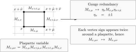
A $\mathbb Z_2$ gauge field assigns a sign to each link. A change at one vertex multiplies both incident plaquette edges by the same $\eta=\pm1$, leaving their product unchanged. Applying this at all four vertices proves plaquette invariance. The local geometry is schematic.

Gauge redundancy is not an ordinary symmetry

The local transformation

$$M_{x,\mu}\mapsto \eta_xM_{x,\mu}\eta_{x+\hat\mu}, \qquad \eta_x=\pm1,$$

is a gauge redundancy. The plaquette variable is invariant because each $\eta_x$ appearing at a corner of the plaquette appears twice:

$$M_{x,\mu\nu}\mapsto M_{x,\mu\nu}.$$

This is different from a global Ising symmetry $\sigma_x\mapsto-\sigma_x$. A global symmetry can be spontaneously broken and can have a local order parameter. A gauge redundancy is a many-to-one description of the same physical configuration. Gauge-dependent quantities, such as a single link expectation value $\langle M_{x,\mu}\rangle$, are not physical observables. In a gauge-invariant formulation they vanish unless a gauge is fixed, and even after gauge fixing their value is not a direct diagnostic of a physical phase.

The local gauge-invariant objects are products around closed boundaries. The smallest one is the plaquette $M_p$. Larger ones are Wilson loops.

The fact that the dual of the three-dimensional Ising model is a gauge theory is already conceptually important. It says that a system with a perfectly ordinary local order parameter can be equivalent, after duality, to a system whose natural probes are nonlocal loop observables. Duality trades one notion of locality for another.

U(1) links and the continuum curl

The $\mathbb Z_2$ gauge system is the discrete cousin of a compact $U(1)$ lattice gauge theory. Replace each sign by a phase,

$$U_{x,\mu}=e^{i\theta_{x,\mu}}, \qquad \theta_{x,\mu}\sim\theta_{x,\mu}+2\pi.$$

When there is a smooth continuum gauge potential, one writes approximately

$$U_{x,\mu}=\exp\left(i a A_\mu\left(x+{a\over2}\hat\mu\right)\right),$$

where $a$ is the lattice spacing. The oriented plaquette product is

$$U_{x,\mu\nu} =U_{x,\mu}U_{x+\hat\mu,\nu}U^{-1}_{x+\hat\nu,\mu}U^{-1}_{x,\nu}.$$

Taking logarithms and expanding at small $a$ gives

$$\log U_{x,\mu\nu} =i\left[\theta_{x,\mu}+\theta_{x+\hat\mu,\nu}-\theta_{x+\hat\nu,\mu}-\theta_{x,\nu}\right] =i a^2 F_{\mu\nu}(x)+O(a^3),$$

with

$$F_{\mu\nu}=\partial_\mu A_\nu-\partial_\nu A_\mu.$$

Thus the plaquette is a small Wilson loop measuring the flux through an elementary square:

$$U_{x,\mu\nu}=\exp\left(i a^2F_{\mu\nu}+O(a^3)\right).$$

A compact Wilson action has the schematic form

$$S_{U(1)}=-K\sum_p\cos\theta_p, \qquad U_p=e^{i\theta_p}.$$

For weak fields,

$$1-\cos\theta_p={\theta_p^2\over2}+O(\theta_p^4) ={a^4\over2}F_{\mu\nu}^2+O(a^5),$$

so the lattice action becomes the Maxwell action in the continuum limit after the usual normalization of $K$ with $a$.

More explicitly, in $d$ dimensions the nonconstant part of the action is

$$S_{U(1)}-S_0 = {K a^{4-d}\over4} \int d^d x\,F_{\mu\nu}F_{\mu\nu}+\cdots.$$

Thus the standard normalization $(4g^2)^{-1}\int F^2$ is obtained by holding $K a^{4-d}=g^{-2}$ fixed in the smooth-field continuum limit. Compact configurations with order-one plaquette angles are not described by this Taylor expansion.

Follow the oriented edges in the figure: opposite sides enter with opposite signs, producing the curl rather than a sum of four potentials.

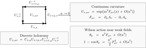
The counterclockwise plaquette product approaches $e^{ia^2F_{\mu\nu}+O(a^3)}$ for a smooth potential and a consistent logarithm branch near zero plaquette angle. Reversing the traversal conjugates the holonomy. The geometry is schematic; the Taylor expansion excludes compact configurations with order-one plaquette angles.

The $\mathbb Z_2$ model keeps only the signs $\pm1$ rather than a continuous phase. But the structural lesson is the same: a gauge field is naturally integrated along links, and its curvature is naturally integrated over plaquettes.

Wilson loops

For a closed lattice contour $C$, define the $\mathbb Z_2$ Wilson loop

$$\boxed{ W(C)=\prod_{\ell\in C}M_\ell. }$$

It is gauge invariant because the gauge signs at every vertex on the closed contour cancel pairwise. If the path were open, the product would transform at its two endpoints and would not be a gauge-invariant observable by itself.

For a compact $U(1)$ theory the Wilson loop is the holonomy

$$W_q(C)=\exp\left(iq\sum_{\ell\in C}\theta_\ell\right) \longrightarrow \exp\left(iq\oint_C A_\mu dx^\mu\right),$$

where $q$ is the charge of the probe. The $\mathbb Z_2$ Wilson loop is the same idea with only two possible phases.

In a compact $U(1)$ theory normalized so that the fundamental electric charge is one, $q$ is an integer. This ensures that the loop is unchanged when a link angle is shifted by $2\pi$.

The strong-coupling expansion of $\langle W(C)\rangle$ is one of the cleanest calculations in lattice gauge theory. Insert $W(C)$ into the high-temperature expansion:

$$\langle W(C)\rangle ={1\over Z_g} \sum_{\{M_\ell\}}\left(\prod_{\ell\in C}M_\ell\right) \prod_p \cosh K_g\left(1+t_gM_p\right).$$

After expanding in plaquettes, a link $\ell$ on the contour $C$ appears once from $W(C)$ and then as many times as selected plaquettes touch it. The sum over $M_\ell$ is nonzero only if the total power is even. Therefore the selected plaquettes no longer form a closed surface. They form a surface whose boundary is $C$:

$$\partial S=C.$$

Hence

$$\langle W(C)\rangle = {\sum_{S:\,\partial S=C} t_g^{A(S)}\over \sum_{S:\,\partial S=0}t_g^{A(S)}}.$$

Suppose $C$ bounds at least one plaquette selection. Let $A_{\min}(C)$ be the smallest number of plaquettes in such a selection and $n_{\min}(C)$ the number of selections attaining that minimum. At fixed finite lattice and contour, the denominator tends to one as $t_g\to0^+$, so

$$\langle W(C)\rangle =n_{\min}(C)t_g^{A_{\min}(C)}[1+o(1)].$$

For a planar rectangle with a unique minimal filling, $n_{\min}=1$. A nonbounding periodic contour has an empty numerator and therefore zero expectation in this finite pure-gauge ensemble. It cannot be assigned a minimal spanning area.

For large bounding rectangles in the strong-coupling phase, the leading area dependence gives a dimensionless lattice string tension $\sigma_{\mathrm{lat}}=-\log t_g+\cdots$. If the lattice spacing is $a$, the physical tension is $\sigma_{\mathrm{phys}}=\sigma_{\mathrm{lat}}/a^2$. Passing from a fixed-contour power series to a large-loop area law requires control of the surface corrections; this calculation alone does not establish continuum confinement. Strong-coupling expansions and Wilson-loop observables develop these separate limits.

In the figure, follow how the loop insertion changes the parity condition on its boundary links.

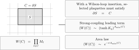
In the finite pure $\mathbb Z_2$ gauge model, a bounding Wilson loop changes the plaquette constraint from $\partial S=0$ to $\partial S=C$. A unique minimal filling contributes $t_g^{A_{\min}}$; multiple minimal fillings contribute their multiplicity. The surface is schematic, with area measured in plaquettes.

Wilson loops as dual disorder loops

Use the cubical ball and fixed exterior spin specified above. Choose a primal plaquette selection $\Sigma$ with $\partial\Sigma=C$. In the dual spin system, define a defect by flipping the sign of every bond crossing $\Sigma$:

$$K_\sigma\sigma_x\sigma_y \longmapsto - K_\sigma\sigma_x\sigma_y \qquad \text{for bonds crossing }\Sigma.$$

If $V$ is the minus-spin cube selection, the unsatisfied bonds now cross $\Sigma+\partial V$, where addition means symmetric difference modulo two. Consequently,

$$\begin{aligned} Z_\sigma[\Sigma] &=e^{K_\sigma N_p}\sum_V e^{-2K_\sigma|\Sigma+\partial V|},\\ \frac{Z_\sigma[\Sigma]}{Z_\sigma[0]} &=\frac{\sum_{\partial S=C}t_g^{|S|}} {\sum_{\partial S=0}t_g^{|S|}} =\langle W(C)\rangle. \end{aligned}$$

This also proves surface independence in its precise domain. If $\Sigma'=\Sigma+\partial V_0$, flipping the spins in $V_0$ permutes the summed configurations and preserves the ratio. The change must respect fixed boundary spins and avoid changing other insertions. On a more general complex, equal boundaries do not suffice: the difference may be a closed surface that does not bound an allowed spin region. Simple connectivity alone is not the required condition.

The figure shows the allowed replacement $\Sigma\mapsto\Sigma+\partial V_0$. It is the three-dimensional counterpart of moving an Ising disorder cut while preserving its endpoints and global sector.

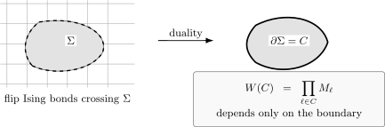
On the cubical ball with fixed exterior spin, flipping dual bonds across $\Sigma$ represents a Wilson loop with $C=\partial\Sigma$. Replacing $\Sigma$ by $\Sigma+\partial V_0$ is undone by flipping the spins in the allowed region $V_0$. Equal boundaries alone do not imply this equivalence on a general topology. This is a schematic projection: the dual bonds cross the faces normally in three dimensions; their projected angles do not represent right angles.

This construction also explains why it is often misleading to ask for “the” local order parameter of a gauge theory. Some phases are best diagnosed by extended probes. In the $\mathbb Z_2$ gauge theory, the large-loop behavior of $\langle W(C)\rangle$ distinguishes the strong-coupling area-law phase from the weak-coupling perimeter-law phase. In the dual spin language, the same transition is the ordinary Ising transition.

Free chiral correlators

Return to the two-dimensional critical Ising theory on the Euclidean plane, away from boundaries and with its vacuum correlators. Write

$$z=x+iy,\qquad \bar z=x-iy,\qquad \partial=\tfrac12(\partial_x-i\partial_y),\qquad \bar\partial=\tfrac12(\partial_x+i\partial_y).$$

The massless action of lessons 9–10 is $\int d^2x\,(u\bar\partial u-v\partial v)$. Define the CFT-normalized fields by

$$\begin{gathered} \psi=\sqrt{2\pi}\,u,\qquad \bar\psi=i\sqrt{2\pi}\,v,\\ S=\frac1{2\pi}\int d^2x\, (\psi\bar\partial\psi+\bar\psi\partial\bar\psi). \end{gathered}$$

Thus the field called $\bar\psi$ here is $-\sqrt{2\pi}$ times the opposite-chirality field called $\bar\psi=-iv$ in lesson 9. The displayed dictionary fixes both the phase and the amplitude. The barred field is an independent Grassmann field, not the complex conjugate of $\psi$.

Their massless equations of motion are

$$\bar\partial\psi=0, \qquad \partial\bar\psi=0,$$

away from operator insertions. The fundamental distribution is $1/z$, with

$$\bar\partial_z {1\over z-w}=\pi\delta^{(2)}(z-w).$$

Writing the action as $\tfrac12\Psi A\Psi$, its chiral kernels are $\bar\partial/\pi$ and $\partial/\pi$. The Grassmann two-point function is $A^{-1}$, so

$$\boxed{ \langle \psi(z)\psi(w)\rangle={1\over z-w}, \qquad \langle \bar\psi(\bar z)\bar\psi(\bar w)\rangle={1\over \bar z-\bar w}, \qquad \langle\psi(z)\bar\psi(\bar w)\rangle=0. }$$

The normalization agrees with Di Francesco, Mathieu, and Sénéchal 1997, § 5.3.2, pp. 129–130, Eqs. (5.88)–(5.93) at their coupling $g=1/(2\pi)$. The pole gives $\psi$ holomorphic weight $h=1/2$, while $\bar\psi$ has antiholomorphic weight $\bar h=1/2$. These are Euclidean plane correlators; lesson 10 distinguishes the algebraic Wick dictionary from the additional analyticity and pole conditions needed for Lorentzian correlators.

Free boson and energy correlators

For a noncompact scalar with action $S_\phi=(8\pi)^{-1}\int d^2x\,(\nabla\phi)^2$, the plane Green function with a chosen additive constant is

$$\langle \phi(z,\bar z)\phi(w,\bar w)\rangle =-\log\!\big(\mu^2|z-w|^2\big).$$

Here $\mu$ is an inverse length. The undifferentiated massless scalar has an infrared zero-mode problem: this expression needs an infrared prescription, or can be used on test functions with zero integral. It is not an unrestricted, infrared-finite scalar vacuum covariance. The logarithm obeys

$$\partial\bar\partial \log |z|^2 =\pi\delta^{(2)}(z).$$

Since $\nabla^2=4\partial\bar\partial$, the stated covariance satisfies $-\nabla^2G=4\pi\delta^{(2)}$. Differentiating it at distinct points gives

$$\langle \partial\phi(z)\partial\phi(w)\rangle =-{1\over (z-w)^2},$$

The minus sign follows from differentiating with respect to both $z$ and $w$. This scalar normalization agrees with Di Francesco, Mathieu, and Sénéchal 1997, § 5.3.1, p. 128, Eqs. (5.73)–(5.77) at their boson coupling $g=1/(4\pi)$. Changing $\mu$ adds a constant and therefore leaves derivative correlators unchanged.

For vertex operators, zero-mode integration imposes charge neutrality, but their finite normal-ordering normalization must also be specified. Neutrality alone does not make separately normalized vertices independent of that choice. The normal-ordering and neutrality construction is developed in Di Francesco, Mathieu, and Sénéchal 1997, § 6.3.2, pp. 161–163. For the related compact-boson zero modes and vertex operators, see the canonical treatment.

For the Ising model, fix the critical energy field in the same CFT normalization:

$$\epsilon=i\psi\bar\psi=-2\pi uv.$$

It is $2\pi$ times the mass-conjugate field $\epsilon_{\rm cont}=-uv$ of lesson 9. The lattice bond also contains an identity contribution and a nonuniversal amplitude; the statement here concerns its connected critical scaling field. Once the chiral poles have been normalized, the factor of $i$ fixes the sign of the energy two-point function.

At separated points, exchanging the two middle fermions supplies a minus sign, which cancels $i^2=-1$. Since mixed chiral contractions vanish, Wick’s theorem gives

$$\langle \epsilon(z,\bar z)\epsilon(w,\bar w)\rangle = \langle \psi(z)\psi(w)\rangle \langle \bar\psi(\bar z)\bar\psi(\bar w)\rangle,$$

so

$$\boxed{ \langle \epsilon(z,\bar z)\epsilon(w,\bar w)\rangle ={1\over |z-w|^2}. }$$

Thus the energy field has scaling dimension

$$\Delta_\epsilon=h_\epsilon+\bar h_\epsilon=1, \qquad h_\epsilon=\bar h_\epsilon={1\over2}.$$

This should be compared with the spin field $\sigma$, whose two-point function at the critical point behaves as

$$\langle \sigma(z,\bar z)\sigma(w,\bar w)\rangle \propto {1\over |z-w|^{1/4}}.$$

The spin field therefore has scaling dimension $\Delta_\sigma=1/8$. Unlike the energy operator, it is not a local polynomial in the free fermion. Transporting the fermion once around a spin insertion changes its sign: the spin is a fermion twist field. The exact weights $h_\sigma=\bar h_\sigma=1/16$ and the half-power fermion–spin operator product are given in Di Francesco, Mathieu, and Sénéchal 1997, § 12.2.2, p. 445, Eqs. (12.23)–(12.26). This is the continuum counterpart of the order–disorder branch cut; it is not a claim that one local insertion specifies every global spin-structure sector.

Summary

The exact spin/gauge identity matches plaquette selections with spin domain walls only after their boundary sectors are matched. A cubical ball with fixed exterior spin supplies an explicit finite example; periodic spin boundaries do not exhaust all closed plaquette cycles.

The gauge variables live on links, and the elementary gauge-invariant field strength is the plaquette product. The local transformation $M_{x,\mu}\mapsto\eta_xM_{x,\mu}\eta_{x+\hat\mu}$ is a redundancy, not an ordinary global symmetry. The natural extended observable is the Wilson loop $W(C)=\prod_{\ell\in C}M_\ell$.

In the strong-coupling expansion, inserting a bounding loop $W(C)$ forces $\partial S=C$. Minimal fillings determine the fixed-loop leading power and its multiplicity; a large-loop area law needs control of the remaining surfaces. In the matched dual spin system, flipping bonds across a spanning surface defines the corresponding disorder loop.

At the two-dimensional critical Ising point, the continuum fermions are free chiral Majorana fields with two-point functions $1/(z-w)$ and $1/(\bar z-\bar w)$. The energy field is the bilinear $\epsilon\sim i\psi\bar\psi$ and has correlator $|z-w|^{-2}$. The spin field has dimension $1/8$ and is a twist field rather than a local fermion bilinear.

Common pitfalls

Gauge redundancy is not symmetry breaking. A gauge transformation is not a physical operation relating different states. It is a redundancy in the variables used to describe one state. Gauge-invariant quantities are closed products such as plaquettes and Wilson loops.

Orientation matters beyond $\mathbb Z_2$. In the $\mathbb Z_2$ theory, link orientation looks irrelevant because $M^{-1}=M$. In $U(1)$ or non-Abelian gauge theory, orientation is essential: reversing a link takes the inverse group element.

The coupling map is not the whole finite-volume identity. The duality relation $e^{-2K_\sigma}=\tanh K_g$ matches singular physics and surface weights, but exact finite-volume partition functions also contain normalization factors and possible topological sectors.

A Wilson loop is an extended probe. It is not the same as a local order parameter. Its large-loop behavior, area law versus perimeter law, diagnoses the gauge phase.

The chiral pole is a distribution. The expression $1/(z-w)$ is not an ordinary function at $z=w$. The contact term in $\bar\partial(1/(z-w))$ is what makes it the inverse of the chiral kinetic operator.

Exercises

Exercise 1: Plaquette gauge invariance

Show explicitly that the $\mathbb Z_2$ plaquette product

$$M_{x,\mu\nu} = M_{x,\mu}M_{x+\hat\mu,\nu}M_{x+\hat\nu,\mu}M_{x,\nu}$$

is invariant under

$$M_{x,\mu}\mapsto \eta_xM_{x,\mu}\eta_{x+\hat\mu}, \qquad \eta_x=\pm1.$$

Solution

Each link in the plaquette transforms as

$$M_{x,\mu}\mapsto \eta_xM_{x,\mu}\eta_{x+\hat\mu},$$ $$M_{x+\hat\mu,\nu}\mapsto \eta_{x+\hat\mu}M_{x+\hat\mu,\nu}\eta_{x+\hat\mu+\hat\nu},$$ $$M_{x+\hat\nu,\mu}\mapsto \eta_{x+\hat\nu}M_{x+\hat\nu,\mu}\eta_{x+\hat\mu+\hat\nu},$$

and

$$M_{x,\nu}\mapsto \eta_xM_{x,\nu}\eta_{x+\hat\nu}.$$

Multiplying all four transformed links gives the original product times

$$\eta_x^2\eta_{x+\hat\mu}^2\eta_{x+\hat\nu}^2\eta_{x+\hat\mu+\hat\nu}^2.$$

Since each $\eta$ is $\pm1$, every square is one. Therefore

$$M_{x,\mu\nu}\mapsto M_{x,\mu\nu}.$$

Exercise 2: Closed surfaces from link sums

Derive the closed-surface constraint in the high-temperature expansion of the $\mathbb Z_2$ gauge partition function

$$Z_g(K_g)=\sum_{\{M_\ell=\pm1\}} \exp\left(K_g\sum_pM_p\right).$$

Solution

Use

$$e^{K_gM_p}=\cosh K_g(1+t_gM_p), \qquad t_g=\tanh K_g.$$

Then

$$Z_g(K_g)=(\cosh K_g)^{N_p} \sum_{\{M_\ell\}} \prod_p(1+t_gM_p).$$

Expanding the product over plaquettes chooses a subset $S$ of plaquettes:

$$\prod_p(1+t_gM_p) =\sum_S t_g^{A(S)}\prod_{p\in S}M_p.$$

Now

$$\prod_{p\in S}M_p =\prod_\ell M_\ell^{n_\ell(S)},$$

where $n_\ell(S)$ is the number of selected plaquettes containing the link $\ell$. The sum over $M_\ell=\pm1$ vanishes unless $n_\ell(S)$ is even. Therefore every link must be touched by an even number of selected plaquettes. This is the condition that $S$ has no boundary:

$$\partial S=0.$$

Each surviving link sum gives two. Retaining every factor,

$$Z_g(K_g)=2^{N_\ell}(\cosh K_g)^{N_p} \sum_{S:\partial S=0}t_g^{|S|}.$$

The closure condition is modulo two and allows intersections. It does not assert that every cycle bounds a cube selection on a periodic lattice.

Exercise 3: Wilson-loop boundary condition

Repeat the previous exercise with a Wilson-loop insertion and show that selected plaquettes must obey $\partial S=C$.

Solution

The numerator of $\langle W(C)\rangle$ is

$$\sum_{\{M_\ell\}}\left(\prod_{\ell\in C}M_\ell\right) \prod_p\cosh K_g(1+t_gM_p).$$

After expanding in plaquettes, a selected surface $S$ contributes

$$t_g^{A(S)} \prod_\ell M_\ell^{n_\ell(S)+\chi_C(\ell)},$$

where $\chi_C(\ell)=1$ if $\ell$ lies on $C$ and $0$ otherwise. The sum over $M_\ell$ is nonzero only if

$$n_\ell(S)+\chi_C(\ell)$$

is even for every link. Hence $n_\ell(S)$ is odd on links of $C$ and even elsewhere. This is exactly the statement that the boundary of the selected plaquette surface is $C$:

$$\partial S=C.$$

If the contour bounds, let $n_{\min}$ count its minimal fillings. The fixed-contour asymptotic is

$$\langle W(C)\rangle =n_{\min}t_g^{A_{\min}(C)}[1+o(1)], \qquad t_g\to0^+.$$

For example, on one cube, a contour bounding three adjacent faces also bounds their complementary three faces. Its exact ratio is $2t_g^3/(1+t_g^6)$, so $n_{\min}=2$. A nonbounding contour has no allowed selection and its numerator vanishes.

Exercise 4: Continuum curvature from a plaquette

For compact $U(1)$ link variables

$$U_{x,\mu}=\exp\left(i a A_\mu\left(x+{a\over2}\hat\mu\right)\right),$$

show that the oriented plaquette product satisfies

$$U_{x,\mu\nu}=\exp\left(i a^2F_{\mu\nu}(x)+O(a^3)\right).$$

Solution

The plaquette product is

$$U_{x,\mu\nu} =U_{x,\mu}U_{x+\hat\mu,\nu}U^{-1}_{x+\hat\nu,\mu}U^{-1}_{x,\nu}.$$

Taking the logarithm gives

$$\log U_{x,\mu\nu} =i a\left[ A_\mu\left(x+{a\over2}\hat\mu\right) +A_\nu\left(x+a\hat\mu+{a\over2}\hat\nu\right) -A_\mu\left(x+a\hat\nu+{a\over2}\hat\mu\right) -A_\nu\left(x+{a\over2}\hat\nu\right) \right].$$

Group the two $A_\nu$ terms and the two $A_\mu$ terms. Taylor expansion at their respective link midpoints gives

$$A_\nu\left(x+a\hat\mu+{a\over2}\hat\nu\right) -A_\nu\left(x+{a\over2}\hat\nu\right) =a\partial_\mu A_\nu(x)+O(a^2),$$

and

$$A_\mu\left(x+a\hat\nu+{a\over2}\hat\mu\right) -A_\mu\left(x+{a\over2}\hat\mu\right) =a\partial_\nu A_\mu(x)+O(a^2).$$

Shifting the derivative evaluation point from a link midpoint to $x$ changes only the displayed $O(a^2)$ remainders.

Therefore

$$\log U_{x,\mu\nu} =i a^2(\partial_\mu A_\nu-\partial_\nu A_\mu)+O(a^3) =i a^2F_{\mu\nu}+O(a^3).$$

Exponentiating gives the desired result.

Exercise 5: Scaling dimension of the Ising energy field

Using

$$\langle\psi(z)\psi(w)\rangle={1\over z-w}, \qquad \langle\bar\psi(\bar z)\bar\psi(\bar w)\rangle={1\over \bar z-\bar w},$$

show that the Ising energy operator $\epsilon\sim i\psi\bar\psi$ has scaling dimension $\Delta_\epsilon=1$.

Solution

By Wick contraction, the sign from exchanging the two middle fermion fields cancels the factor $i^2=-1$, so up to the chosen normalization,

$$\langle \epsilon(z,\bar z)\epsilon(w,\bar w)\rangle \propto \langle\psi(z)\psi(w)\rangle \langle\bar\psi(\bar z)\bar\psi(\bar w)\rangle.$$

Substituting the chiral two-point functions gives

$$\langle \epsilon(z,\bar z)\epsilon(w,\bar w)\rangle \propto {1\over (z-w)(\bar z-\bar w)} ={1\over |z-w|^2}.$$

For a scalar primary of scaling dimension $\Delta$, the two-point function scales as

$$\langle O(z,\bar z)O(w,\bar w)\rangle\propto {1\over |z-w|^{2\Delta}}.$$

Comparing with $|z-w|^{-2}$ gives

$$2\Delta_\epsilon=2, \qquad \Delta_\epsilon=1.$$

Equivalently, $\psi$ has weights $(1/2,0)$ and $\bar\psi$ has weights $(0,1/2)$, so $\epsilon\sim i\psi\bar\psi$ has weights $(1/2,1/2)$ and total dimension $1$.

References

• P. Di Francesco, P. Mathieu, and D. Sénéchal, Conformal Field Theory. Graduate Texts in Contemporary Physics, Springer, New York (1997). DOI.
• F. J. Wegner, “Duality in generalized Ising models.” Les Houches summer-school contribution, arXiv:1411.5815v1 [hep-lat] (2014). Stable record; Open PDF.

Further reading

• L. P. Kadanoff and H. Ceva, “Determination of an Operator Algebra for the Two-Dimensional Ising Model.” Physical Review B 3, 3918–3939 (1971). DOI. The order–disorder construction underlying the preceding lessons.
• J. B. Kogut, “An Introduction to Lattice Gauge Theory and Spin Systems.” Reviews of Modern Physics 51, 659–713 (1979). DOI. Lattice expansions, gauge observables and duality.
• A. M. Polyakov, Gauge Fields and Strings. Contemporary Concepts in Physics, vol. 3, Harwood Academic Publishers (1987). DOI. Statistical field theory, disorder variables and confinement.
• F. J. Wegner, “Duality in Generalized Ising Models and Phase Transitions without Local Order Parameters.” Journal of Mathematical Physics 12, 2259–2272 (1971). DOI. The original generalized-duality construction.
• K. G. Wilson, “Confinement of Quarks.” Physical Review D 10, 2445–2459 (1974). DOI. Lattice gauge theory and the Wilson-loop confinement criterion.