Disorder Lines, Branch Cuts, and Defect Operators

An Ising disorder operator is the endpoint of a line across which the signs of the couplings are reversed. At zero magnetic field, a contractible change of the line’s route can be undone by an exact change of spin variables that preserves the boundary conditions. Within that class of deformations, its endpoints and its crossings with spin insertions carry the observable information. This is the lattice origin of a local twist field with $\mathbb Z_2$ monodromy.

The central result is exact: such a deformation through empty space leaves the partition function unchanged, while a deformation across one order operator multiplies the mixed correlator by $-1$. We will prove both statements directly and then reinterpret the line as a branch cut and a topological symmetry defect.

Two short comparisons connect Ising defects to extended observables in gauge theory and gravity, and distinguish the Ising disorder field from random impurities and Anderson localization. Neither comparison is needed to define $\mu$.

Required background. Fixed points, tricriticality, and order–disorder variables introduces the Ising order field and the first order–disorder dictionary. Ising graphical expansions supplies the even-subgraph expansion used below.

Helpful background. Kramers–Wannier duality explains why the disorder field orders on the opposite side of the transition from the spin field.

The lattice disorder insertion

Consider the zero-field nearest-neighbor Ising model on a finite simply connected square-lattice region with free boundary spins,

$$\begin{gathered} Z(K)=\sum_{\{\sigma\}} \exp\!\left(K\sum_{\langle ij\rangle}\sigma_i\sigma_j\right),\\ \sigma_i=\pm1, \qquad K>0. \end{gathered}$$

Let $\Gamma$ be a path on the dual lattice. It crosses a set of bonds of the original lattice. Introduce a bond-sign background

$$\eta_{ij}^{(\Gamma)}= \begin{cases} -1, & \langle ij\rangle\text{ is crossed by }\Gamma,\\ +1, & \text{otherwise}, \end{cases}$$

and define

$$Z_\Gamma(K)=\sum_{\{\sigma\}} \exp\!\left( K\sum_{\langle ij\rangle} \eta_{ij}^{(\Gamma)}\sigma_i\sigma_j \right).$$

Thus every crossed bond has $K\mapsto-K$. Relative to the unmodified Boltzmann weight, one crossed bond inserts

$${e^{-K\sigma_i\sigma_j}\over e^{K\sigma_i\sigma_j}} =e^{-2K\sigma_i\sigma_j},$$

and a whole path inserts

$$\prod_{\langle ij\rangle\perp\Gamma} e^{-2K\sigma_i\sigma_j}.$$

If $\Gamma$ joins dual sites $p^*$ and $q^*$, the exact lattice definition is

$$\boxed{ \langle\mu(p^*)\mu(q^*)\rangle_{\rm lat} ={Z_\Gamma(K)\over Z(K)}. }$$

This is the partition-function definition of Kadanoff and Ceva 1971, § II A, p. 3919, Eqs. (2.1)–(2.3). It fixes the lattice normalization. A continuum scaling field may later be multiplied by a cutoff-dependent renormalization factor. A single disorder insertion is possible only after its cut is continued to a boundary or to infinity; on a closed finite lattice, disorder endpoints occur in pairs.

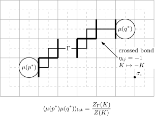
The dual path $\Gamma$ crosses original-lattice bonds. Each crossing reverses one coupling, $K\mapsto-K$. Its dual endpoints are the disorder insertions $\mu(p^*)$ and $\mu(q^*)$.

The definition is sometimes described as an antiferromagnetic seam. That phrase is useful microscopically, but it should not suggest that the seam itself is a rigid physical string. Its shape is redundant under the allowed deformations.

Endpoint flux and path independence

Suppose $\Gamma$ and $\Gamma'$ have the same endpoints and differ by the boundary of a set $R$ of original-lattice sites. With the stated free boundary all spins are summed; if boundary spins are instead fixed, restrict $R$ so that their values are unchanged. Define

$$\rho_i= \begin{cases} -1, & i\in R,\\ +1, & i\notin R. \end{cases}$$

The two bond-sign backgrounds obey

$$\eta_{ij}^{(\Gamma')} =\rho_i\eta_{ij}^{(\Gamma)}\rho_j.$$

Now make the bijective change of summation variables

$$\sigma_i'=\rho_i\sigma_i.$$

Then

$$\eta_{ij}^{(\Gamma')}\sigma_i\sigma_j =\eta_{ij}^{(\Gamma)}\sigma_i'\sigma_j',$$

so term by term after relabeling configurations,

$$\boxed{Z_{\Gamma'}(K)=Z_\Gamma(K).}$$

The physical data carried by $\eta$ can be read from the plaquette product

$$W_{r^*}=\prod_{\langle ij\rangle\in\partial r^*}\eta_{ij}.$$

For a path ending at $p^*$ and $q^*$,

$$\begin{aligned} W_{p^*}=W_{q^*}&=-1,\\ W_{r^*}&=+1\qquad(r^*\ne p^*,q^*). \end{aligned}$$

The individual negative bonds move under $\eta_{ij}\mapsto\rho_i\eta_{ij}\rho_j$, but the endpoint fluxes do not. In this precise lattice sense, $\mu$ inserts $\mathbb Z_2$ flux.

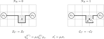
Changing $\Gamma$ to $\Gamma'$ is equivalent to flipping every dummy spin in the swept region $R$. With no spin insertion in $R$, nothing changes. A spin insertion in $R$ contributes one extra minus sign.

There is one important topological qualification. On a torus, two paths with the same endpoints need not differ by the boundary of a region: they may differ by a noncontractible cycle. Such a change alters the global spin boundary-condition sector. Local path independence therefore means invariance under contractible deformations that preserve the boundary data and avoid charged insertions Polyakov 1987, § 10.3.1, p. 276.

Order fields detect the cut

Insert spins at sites $i_1,\ldots,i_n$ and use the disorder background $\Gamma$:

$$\begin{aligned} \mathcal C_\Gamma &= {1\over Z(K)} \sum_{\{\sigma\}} \left(\prod_{a=1}^n\sigma_{i_a}\right)\\ &\quad\times \exp\!\left( K\sum_{\langle ij\rangle} \eta_{ij}^{(\Gamma)}\sigma_i\sigma_j \right). \end{aligned}$$

Under the same variable change,

$$\sigma_{i_a}=\rho_{i_a}\sigma_{i_a}',$$

and therefore

$$\boxed{ \begin{gathered} \mathcal C_{\Gamma'} =(-1)^{N_R}\mathcal C_\Gamma,\\ N_R=\#\{a:i_a\in R\}\pmod2. \end{gathered} }$$

A deformation through one spin gives $-1$; a deformation through two spins gives $+1$. This is mutual nonlocality: $\sigma$ and $\mu$ can each be treated as local fields in an appropriate description, but a mixed correlator needs branch-cut data.

The sign is determined by $\mathbb Z_2$ charge, not by whether an insertion happens to sit near the line. An even local operator, such as the continuum energy field or a suitably defined bond-energy insertion, does not acquire this monodromy. If the deformation changes which bond defines a lattice energy operator, one must first transport that operator consistently; the invariant statement is that a $\mathbb Z_2$-even local field has trivial linking with the symmetry defect.

Branch points and monodromy

The complex logarithm provides a useful comparison:

$$\log z=\int_1^z {d\zeta\over\zeta}.$$

Changing the integration path without winding around the origin changes nothing. Winding once gives

$$\log z\longmapsto\log z+2\pi i.$$

The drawn cut is conventional, but the monodromy around the branch point is not. The Ising cut works the same way, except that its monodromy is a sign. In a mixed correlator,

$$\boxed{ \begin{gathered} \sigma\ \text{continued once around}\ \mu\\ \Longrightarrow \sigma\mapsto-\sigma. \end{gathered} }$$

Equivalently, with a chosen cut from the origin,

$$\sigma(e^{2\pi i}z)\mu(0) =-\sigma(z)\mu(0).$$

This last equation records analytic continuation of a correlator. It is not an equality between two ordinary single-valued functions.

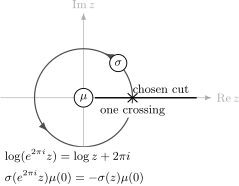
The position of the cut is a convention. Transporting $\sigma$ once around the branch point $\mu$ necessarily has odd intersection parity with the cut and produces the physical monodromy $-1$.

The loop expansion measures intersection parity

The high-temperature expansion makes the same topology algebraic. For every bond,

$$\begin{gathered} e^{K\eta_{ij}\sigma_i\sigma_j} =\cosh K\left(1+t\eta_{ij}\sigma_i\sigma_j\right),\\ t=\tanh K. \end{gathered}$$

Choose either the $1$ or the second term on each bond. A chosen subgraph $C$ survives the spin sum only if an even number of chosen bonds meet at every site. Hence $C$ is an even subgraph, a union of closed loops, and

$$\sum_{\{\sigma\}} \prod_{\langle ij\rangle\in C}\sigma_i\sigma_j =2^{N_s}.$$

The disorder background contributes

$$\prod_{\langle ij\rangle\in C}\eta_{ij}^{(\Gamma)} =(-1)^{I(C,\Gamma)},$$

where $I(C,\Gamma)$ is the number of primal-bond/dual-path intersections modulo $2$. Therefore

$$\boxed{ \begin{aligned} Z_\Gamma(K) &=2^{N_s}(\cosh K)^{N_b}\\ &\quad\times\sum_{C:\,\partial C=0} t^{|C|}(-1)^{I(C,\Gamma)}. \end{aligned} }$$

Dividing by the same loop sum without the sign gives

$${Z_\Gamma(K)\over Z(K)} =\left\langle(-1)^{I(C,\Gamma)}\right\rangle_{\rm loops}.$$

For a closed loop $C$ on the plane, odd intersection means that $C$ separates the two endpoints of $\Gamma$. This criterion depends on the endpoints, not on the detailed route of the cut.

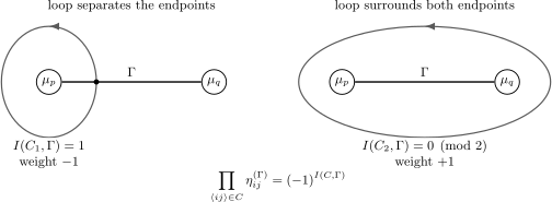
Every high-temperature loop configuration is weighted by $(-1)^{I(C,\Gamma)}$. A loop surrounding one endpoint has odd parity; a loop surrounding both endpoints has even parity.

Order and disorder in the two phases

Kramers–Wannier duality defines the dual coupling by

$$\begin{gathered} e^{-2K^*}=\tanh K,\\ \sinh 2K\,\sinh 2K^*=1. \end{gathered}$$

With compatible normalizations, the disorder correlator at $K$ is the spin correlator of the dual model at $K^*$. The phase pattern then follows without guessing:

• for $K>K_c$, the spins have long-range order while the disorder correlator decays exponentially;
• for $K<K_c$, the spin correlator decays exponentially while the disorder field has long-range order;
• at the self-dual critical point, both correlators are power laws and order and disorder have the same scaling dimension.

At infinite temperature, $K=0$, changing bond signs does nothing, so the lattice normalization above gives

$$\langle\mu(p^*)\mu(q^*)\rangle_{K=0}=1.$$

Deep in the ordered phase, the endpoints force a domain-wall segment and the large-separation behavior has the form

$$\langle\mu(p^*)\mu(q^*)\rangle \sim e^{-|p^*-q^*|/\xi_\mu}.$$

This is the precise sense in which $\mu$ is a disorder parameter: it orders where $\sigma$ disorders.

Closed symmetry defects and extended observables

Close the dual path into a contractible loop $C$. Flipping every spin inside removes the seam. If local fields $O_a$ of $\mathbb Z_2$ charges $q_a\in\{0,1\}$ lie inside, the same variable change gives

$$\begin{aligned} &\left\langle U(C)\prod_a O_a(x_a)\right\rangle\\ &\qquad=(-1)^{\sum_{x_a\,{\rm inside}\,C}q_a} \left\langle\prod_a O_a(x_a)\right\rangle. \end{aligned}$$

Thus a closed disorder line implements the global spin-flip symmetry on the operators it surrounds. It is topological under deformations that do not cross charged insertions. Opening this invertible symmetry line creates twist endpoints, the disorder fields.

This example shows why a local action does not list every useful observable. For a non-Abelian gauge connection,

$$F_{\mu\nu} =\partial_\mu A_\nu-\partial_\nu A_\mu -ig[A_\mu,A_\nu],$$

so $\operatorname{tr}F^2$ contains quadratic, cubic, and quartic gauge-field terms. Expanding the Einstein–Hilbert action about flat space similarly produces self-interactions of the metric perturbation. Yet Wilson lines, magnetic disorder lines, boundary conditions, and other extended insertions carry information not captured by merely listing local interaction vertices. The Ising seam is a finite-sum model of that distinction.

Random disorder and the diffusion pole

The word “disorder” now changes meaning. An Ising disorder operator is a controlled twist insertion. Random disorder means spatially varying couplings or potentials drawn from an ensemble. The two notions are logically independent.

Consider one small conserved-density disturbance $n(t,x)$ about homogeneous equilibrium, with constant $D>0$, no drift, and no mixing with another slow mode. With constitutive law $j=-D\nabla n$, the continuity equation gives

$$\partial_t n=D\nabla^2n.$$

Using the site-wide inverse plane-wave phase $e^{-ip\cdot x}=e^{-i\omega t+i\mathbf k\cdot\mathbf x}$, the inverse diffusion operator is

$$G_{\rm diff}(\omega,k) ={1\over-i\omega+Dk^2},$$

and its pole is

$$\omega_*=-iDk^2.$$

Because $\omega_*\to0$ as $k\to0$, long-wavelength density disturbances relax slowly. To distinguish the causal response from the retarded commutator, couple a chemical-potential source by

$$\begin{aligned} H_{\rm ext}(t)&=-\int d^{d_s}x\,\mu_{\rm ext}(t,x)\widehat n(x),\\ G_{nn}^{R}(t,x)&=-i\theta(t)\langle[\widehat n(t,x),\widehat n(0,0)]\rangle. \end{aligned}$$

Here $\widehat n$ is the density operator and $n=\delta\langle\widehat n\rangle$. First-order Hamiltonian perturbation theory gives $n=\mathcal R_{nn}\mu_{\rm ext}$ with $\mathcal R_{nn}=-G_{nn}^{R}$ for this source-independent operator. Conservation and the static susceptibility $\chi>0$ then give

$$\begin{aligned} \mathcal R_{nn}(\omega,k)&=\chi\,{Dk^2\over Dk^2-i\omega},\\ G_{nn}^{R}(\omega,k)&=-\chi\,{Dk^2\over Dk^2-i\omega}. \end{aligned}$$

The sign follows from the source convention; a local contact cannot reverse the nonlocal pole residue. Kovtun 2012, § 2.1, pp. 16–18, arXiv v1, Open PDF derives this same density response. The canonical Hamiltonian-source derivation fixes the sign, and the scalar Einstein relation explains $D=\sigma/\chi$ and its single-density regime. Confusing the inverse diffusion operator with either full density kernel also loses the important $k^2$ numerator.

For the constant-$D$ model on the whole line, a localized excess $N>0$ at $x_0$ has the heat-kernel solution

$$n(x,t)=\frac{N}{\sqrt{4\pi Dt}} \exp\!\left[-\frac{(x-x_0)^2}{4Dt}\right], \qquad t>0.$$

Its total weight is $\int n\,dx=N$, its mean is $N^{-1}\int xn\,dx=x_0$, and its variance is $2Dt$. Diffusion broadens the packet without translating its center. The point-source solution is exact for this ideal differential equation; a microscopic hydrodynamic description applies only after coarse graining beyond its short time and length scales. In the figure, compare the stationary peaks and equal full-line areas before examining the common causal pole.

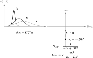
Constant-$D$ diffusion on the whole line, with no drift or boundaries. The upper panel plots $f=\ell n/N$ against $u=(x-x_0)/\ell$ at $s=Dt/\ell^2=1/8,3/10,7/10$; the exact full-line curves have unit area, zero mean, and variance $2s$. Only the displayed window is truncated. The lower panel is schematic: for nonzero $k$, $\omega_*=-iDk^2$ approaches the origin as $k\to0$. With the stated Hamiltonian source, $\mathcal R_{nn}=-G_{nn}^{R}$; both kernels have the conserved-density numerator $Dk^2$.

For noninteracting particles with time-reversal symmetry and no spin-orbit coupling, the standard orthogonal localization class has no true metallic phase in two dimensions: interference drives the large-scale conductance downward. In three dimensions an unstable metal–insulator critical point can separate diffusive and localized phases. These statements have symmetry-class and interaction qualifications; they are not universal claims about every two-dimensional disordered system. Heuristically, localization corresponds to a scale- and frequency-dependent diffusion constant tending to zero in the infrared, not to the Ising twist field $\mu$.

From disorder endpoint to lattice fermion

The construction has established three exact pieces of data:

1. $\mu$ is an endpoint flux, so its cut is movable by a spin-variable change.
2. A spin insertion linked once with that cut contributes a sign $-1$.
3. The same sign is the mod-$2$ intersection number in the loop expansion.

The next step is to bring an order insertion and a disorder endpoint to neighboring primal and dual sites. Rotating that point-split pair by $2\pi$ forces one order–disorder crossing, so the composite is antiperiodic. That is how a spinor emerges from commuting Ising spins.

Common pitfalls

Treating the cut as a physical string. Its endpoints and global homology class are physical; a contractible deformation of its route is a change of spin variables.

Claiming complete path independence in a mixed correlator. The magnitude is unchanged, but crossing an odd number of $\mathbb Z_2$-odd insertions changes the sign.

Ignoring global topology. On a torus, adding a noncontractible seam changes the boundary-condition sector and cannot be removed by a local spin flip.

Equating the two meanings of disorder. The twist field $\mu$ and quenched random impurities are different constructions. The diffusion discussion is a comparison, not part of the Ising definition.

Exercises

Exercise 1: deforming the seam

Let $\Gamma$ and $\Gamma'$ have the same endpoints and differ by the boundary of a site set $R$. Prove $Z_{\Gamma'}=Z_\Gamma$. Then repeat the proof with $n$ spin insertions and obtain the sign $(-1)^{N_R}$.

Solution

Set $\rho_i=-1$ in $R$ and $+1$ outside. Every bond crossing $\partial R$ receives one factor of $-1$, while every other bond receives zero or two. Hence

$$\eta_{ij}^{(\Gamma')}=\rho_i\eta_{ij}^{(\Gamma)}\rho_j.$$

The bijection $\sigma_i'=\rho_i\sigma_i$ maps the $\Gamma'$ Boltzmann weight to the $\Gamma$ weight, proving equality of partition functions. With insertions,

$$\prod_{a=1}^n\sigma_{i_a} =\left(\prod_{a=1}^n\rho_{i_a}\right) \prod_{a=1}^n\sigma_{i_a}',$$

and the prefactor is $(-1)^{N_R}$.

Exercise 2: endpoint flux

Show that a dual path has $W_{p^*}=W_{q^*}=-1$ at its two endpoints and $W=+1$ elsewhere. Show directly that $W$ is invariant under $\eta_{ij}\mapsto\rho_i\eta_{ij}\rho_j$.

Solution

At an interior dual vertex, the path enters and exits, so it crosses the plaquette boundary twice and contributes $(-1)^2=+1$. At an endpoint it crosses the boundary once, giving $-1$. Under the transformation, every site on a plaquette boundary occurs in exactly two adjacent bonds, so all $\rho_i$ factors square to one:

$$\prod_{\langle ij\rangle\in\partial p^*} \rho_i\eta_{ij}\rho_j =\prod_{\langle ij\rangle\in\partial p^*}\eta_{ij}.$$

Exercise 3: loop-intersection formula

Derive

$$\begin{aligned} Z_\Gamma &=2^{N_s}(\cosh K)^{N_b}\\ &\quad\times\sum_{C:\,\partial C=0} (\tanh K)^{|C|}(-1)^{I(C,\Gamma)}. \end{aligned}$$

Why does a local deformation of $\Gamma$ leave every term unchanged?

Solution

Expand each bond factor as

$$\cosh K(1+t\eta_{ij}\sigma_i\sigma_j).$$

The spin sum vanishes at any site incident on an odd number of selected bonds, so only even subgraphs remain. Each surviving spin sum is $2^{N_s}$, each selected bond gives $t$, and each selected bond crossing $\Gamma$ gives $-1$. A contractible deformation changes the intersection number of any closed subgraph by an even integer, so its parity and weight are unchanged.

Exercise 4: the conserved-density numerator

Use the Hamiltonian source and retarded convention defined above, with constant $D,\chi>0$, and the constitutive law

$$j=-D\chi\nabla\!\left({n\over\chi}-\mu_{\rm ext}\right).$$

Derive the response $n=\mathcal R_{nn}\mu_{\rm ext}$ and the retarded correlator $G_{nn}^R$. Check the static and homogeneous limits, and the sign of the diagonal spectral weight $\rho_{nn}=-2\operatorname{Im}G_{nn}^R$.

Solution

Continuity gives

$$\partial_t n-D\nabla^2n=-D\chi\nabla^2\mu_{\rm ext}.$$

Fourier transformation yields

$$(-i\omega+Dk^2)n =D\chi k^2\mu_{\rm ext},$$

so

$$\begin{aligned} \mathcal R_{nn}(\omega,k)&=\chi\frac{Dk^2}{Dk^2-i\omega},\\ G_{nn}^R(\omega,k)&=-\mathcal R_{nn}(\omega,k). \end{aligned}$$

Taking $\omega\to0$ at fixed nonzero $k$ gives $\mathcal R_{nn}(0,k)=\chi$ and $G_{nn}^R(0,k)=-\chi$. Taking $k\to0$ first at fixed nonzero $\omega$ instead gives zero response: a spatially uniform time-dependent chemical potential cannot change the total conserved charge of the isolated system. These paths to the origin differ; equilibration with a reservoir is a different source protocol.

For real nonzero frequency,

$$\rho_{nn}(\omega,k) =\frac{2\chi Dk^2\omega}{(Dk^2)^2+\omega^2}, \qquad \frac{\rho_{nn}(\omega,k)}{\omega}\ge0.$$

Thus the diagonal spectral weight has the passive-equilibrium sign. Using the positive response itself as the minus-$i$ retarded commutator would give the wrong sign while leaving the pole location unchanged.

References

• E. Abrahams, P. W. Anderson, D. C. Licciardello, and T. V. Ramakrishnan, “Scaling Theory of Localization: Absence of Quantum Diffusion in Two Dimensions,” Physical Review Letters 42, 673–676 (1979), doi:10.1103/PhysRevLett.42.673.
• L. P. Kadanoff and H. Ceva, “Determination of an Operator Algebra for the Two-Dimensional Ising Model,” Physical Review B 3, 3918–3939 (1971), doi:10.1103/PhysRevB.3.3918.
• Pavel Kovtun, “Lectures on Hydrodynamic Fluctuations in Relativistic Theories,” Journal of Physics A: Mathematical and Theoretical 45, 473001 (2012). DOI. Open PDF, arXiv v1.
• H. A. Kramers and G. H. Wannier, “Statistics of the Two-Dimensional Ferromagnet. Part I,” Physical Review 60, 252–262 (1941), doi:10.1103/PhysRev.60.252.
• Alexander M. Polyakov, Gauge Fields and Strings. Contemporary Concepts in Physics, Vol. 3. Harwood Academic Publishers, 1987. DOI.

Further reading

• P. Di Francesco, P. Mathieu, and D. Sénéchal, Conformal Field Theory. Graduate Texts in Contemporary Physics. Springer, 1997, Chapters 4 and 12.
• B. M. McCoy and T. T. Wu, The Two-Dimensional Ising Model. Harvard University Press, 1973.