Klein–Gordon Equation and Scalar Modes

The previous page solved a free nonrelativistic field by diagonalizing it into momentum modes. Each mode carried energy $\boldsymbol p^2/(2m)$ and had an occupation number. The relativistic free theory should look similar at the level of particles: a mode of momentum $\boldsymbol p$ should carry energy

$$\omega_{\boldsymbol p}=\sqrt{\boldsymbol p^2+m^2}.$$

But there is a catch. If we simply replace the nonrelativistic one-particle Hamiltonian $-\nabla^2/(2m)$ by the square-root operator $\sqrt{-\nabla^2+m^2}$, the result is awkward and nonlocal in position space. Relativistic field theory takes a better route: it uses a local field equation whose plane-wave solutions automatically obey the relativistic dispersion relation.

That local equation is the Klein–Gordon equation,

$$(\partial_t^2-\nabla^2+m^2)\phi(x)=0.$$

The price is that the equation is second order in time. The reward is locality, Lorentz covariance, and an oscillator interpretation: each momentum mode obeys an oscillator equation, with a genuine harmonic oscillator when $\omega_{\boldsymbol p}>0$.

Relativistic dispersion from a local equation

Scalar oscillator-mode normalization

The shorthand

$$\int_{\boldsymbol p}\equiv\int\frac{d^3p}{(2\pi)^3}$$

is used in continuum mode expansions.

The canonical derivation below uses oscillator-normalized operators,

$$[a_{\boldsymbol p},a_{\boldsymbol q}^\dagger]=(2\pi)^3\delta^{(3)}(\boldsymbol p-\boldsymbol q),$$

with the familiar $1/\sqrt{2\omega_{\boldsymbol p}}$ in the field expansion. This is equivalent to the qft.org covariant normalization by defining

$$A(\boldsymbol p)=\sqrt{2\omega_{\boldsymbol p}}\,a_{\boldsymbol p}, \qquad [A(\boldsymbol p),A^\dagger(\boldsymbol q)] =(2\pi)^3 2\omega_{\boldsymbol p}\delta^{(3)}(\boldsymbol p-\boldsymbol q).$$

Then the same field can be written with the invariant measure $d^3p/[(2\pi)^3 2\omega_{\boldsymbol p}]$.

Start with a real scalar field $\phi(\boldsymbol x,t)$. A plane wave with four-momentum $p^\mu=(p^0,\boldsymbol p)$ is written as

$$\phi(x)=e^{-ip\cdot x}=e^{-ip^0t+i\boldsymbol p\cdot\boldsymbol x}.$$

Acting on this wave,

$$\partial_t^2\phi=-(p^0)^2\phi, \qquad \nabla^2\phi=-\boldsymbol p^2\phi.$$

Therefore

$$(\Box+m^2)\phi =\left(-(p^0)^2+\boldsymbol p^2+m^2\right)\phi.$$

The equation $(\Box+m^2)\phi=0$ gives

$$(p^0)^2=\boldsymbol p^2+m^2.$$

Thus the allowed frequencies are

$$p^0=\pm\omega_{\boldsymbol p}, \qquad \omega_{\boldsymbol p}=\sqrt{\boldsymbol p^2+m^2}.$$

Equivalently,

$$p_\mu p^\mu=m^2.$$

This is the relativistic mass-shell condition. The positive-energy sheet describes particles with energy $+\omega_{\boldsymbol p}$. The negative-frequency solutions are not discarded; in field theory they become part of the operator expansion and are tied to creation operators.

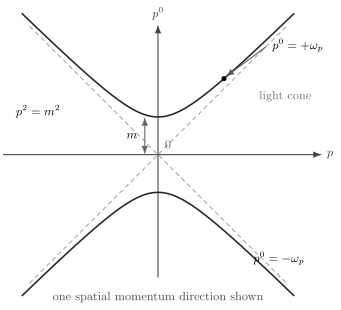
A one-dimensional slice through the mass shell $p^2=m^2$. The Klein–Gordon equation permits both $p^0=+\omega_{\boldsymbol p}$ and $p^0=-\omega_{\boldsymbol p}$ as frequencies, but the quantized field has a positive Hamiltonian after the modes are interpreted as creation and annihilation operators.

The important point is not merely that the dispersion relation is relativistic. It is that the dispersion relation came from a differential operator that is local in spacetime. Locality is the structural reason the Klein–Gordon equation is preferable to a square-root Schrödinger equation.

The action and the Hamiltonian

The Klein–Gordon equation follows from the Lorentz-invariant action

$$S=\int d^4x\,\mathcal L, \qquad \mathcal L=\frac12\partial_\mu\phi\,\partial^\mu\phi-\frac12m^2\phi^2.$$

In space-plus-time notation,

$$\mathcal L=\frac12\dot\phi^2-\frac12(\nabla\phi)^2-\frac12m^2\phi^2.$$

To derive the interior equation, take smooth variations $\phi\to\phi+\delta\phi$ with compact support in the spacetime interior. A boundary-value problem instead needs allowed boundary variations and any boundary action chosen so that the surface variation vanishes; see scalar boundary data. For the compactly supported variations,

$$\begin{aligned} \delta S &=\int d^4x\, \left(\partial_\mu\phi\,\partial^\mu\delta\phi-m^2\phi\,\delta\phi\right) \\ &=-\int d^4x\,\delta\phi\,(\partial_\mu\partial^\mu+m^2)\phi, \end{aligned}$$

where the boundary term vanishes by the support assumption. Since $\delta\phi$ is arbitrary in the interior,

$$(\Box+m^2)\phi=0.$$

The canonical momentum is

$$\pi(\boldsymbol x,t)=\frac{\partial\mathcal L}{\partial\dot\phi}=\dot\phi(\boldsymbol x,t).$$

The Hamiltonian density is

$$\mathcal H=\pi\dot\phi-\mathcal L =\frac12\pi^2+\frac12(\nabla\phi)^2+\frac12m^2\phi^2.$$

Therefore

$$H=\int d^3x\,\frac12\left(\pi^2+(\nabla\phi)^2+m^2\phi^2\right).$$

This Hamiltonian is positive for a real classical field. That fact will survive quantization, up to the usual zero-point energy.

Momentum modes are harmonic oscillators

Fourier-transform the field in space,

$$\phi(\boldsymbol x,t)=\int_{\boldsymbol p}\phi_{\boldsymbol p}(t)e^{i\boldsymbol p\cdot\boldsymbol x}.$$

The Klein–Gordon equation becomes

$$\ddot\phi_{\boldsymbol p}(t)+(\boldsymbol p^2+m^2)\phi_{\boldsymbol p}(t)=0.$$

Thus each momentum mode satisfies

$$\ddot\phi_{\boldsymbol p}+\omega_{\boldsymbol p}^2\phi_{\boldsymbol p}=0, \qquad \omega_{\boldsymbol p}=\sqrt{\boldsymbol p^2+m^2}.$$

For $m>0$, every mode has positive frequency, giving the oscillator structure used in the quantum construction below. The frequencies are fixed by the relativistic mass shell.

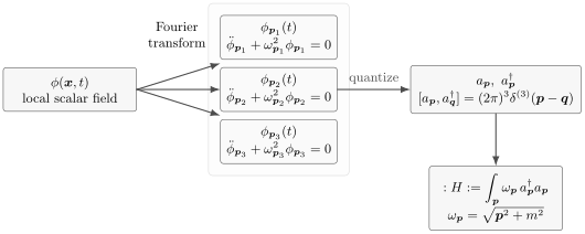
The local field $\phi(\boldsymbol x,t)$ is equivalent, after Fourier transformation, to independent oscillator modes $\phi_{\boldsymbol p}(t)$. Each mode has frequency $\omega_{\boldsymbol p}=\sqrt{\boldsymbol p^2+m^2}$.

For a real field, $\phi_{-\boldsymbol p}=\phi_{\boldsymbol p}^*$ classically, so the variables at $\boldsymbol p$ and $-\boldsymbol p$ are not independent. The compact operator expansion below handles this reality condition automatically.

Canonical quantization of the real scalar field

For this quantum construction, take $m>0$ and select the positive-frequency branch $\omega_{\boldsymbol p}>0$. The free vacuum is annihilated by every $a_{\boldsymbol p}$. Point fields below are operator-valued distributions, and momentum kets are generalized states; their continuum formulas are interpreted after suitable smearing. This scope leaves the later classical massless example intact.

Canonical quantization imposes the continuum equal-time commutation relations as distributional identities:

$$[\phi(\boldsymbol x,t),\pi(\boldsymbol y,t)]=i\delta^{(3)}(\boldsymbol x-\boldsymbol y),$$

and

$$[\phi(\boldsymbol x,t),\phi(\boldsymbol y,t)]=0, \qquad [\pi(\boldsymbol x,t),\pi(\boldsymbol y,t)]=0.$$

The mode expansion that realizes these commutators is

$$\phi(\boldsymbol x,t) =\int_{\boldsymbol p}\frac{1}{\sqrt{2\omega_{\boldsymbol p}}} \left( a_{\boldsymbol p}e^{-i\omega_{\boldsymbol p}t+i\boldsymbol p\cdot\boldsymbol x} +a_{\boldsymbol p}^\dagger e^{i\omega_{\boldsymbol p}t-i\boldsymbol p\cdot\boldsymbol x} \right),$$

In terms of the spatial Fourier coefficient introduced above, the same expansion reads

$$\phi_{\boldsymbol p}(t) =\frac{1}{\sqrt{2\omega_{\boldsymbol p}}} \left( a_{\boldsymbol p}e^{-i\omega_{\boldsymbol p}t} +a_{-\boldsymbol p}^\dagger e^{i\omega_{\boldsymbol p}t} \right).$$

The momentum reversal on the creation operator is essential: it gives

$$\phi_{\boldsymbol p}^\dagger(t)=\phi_{-\boldsymbol p}(t),$$

which is the Fourier-space form of the reality condition $\phi^\dagger(x)=\phi(x)$.

The conjugate momentum is

$$\pi(\boldsymbol x,t)=\dot\phi(\boldsymbol x,t) =\int_{\boldsymbol p} \left(-i\sqrt{\frac{\omega_{\boldsymbol p}}{2}}\right) \left( a_{\boldsymbol p}e^{-i\omega_{\boldsymbol p}t+i\boldsymbol p\cdot\boldsymbol x} -a_{\boldsymbol p}^\dagger e^{i\omega_{\boldsymbol p}t-i\boldsymbol p\cdot\boldsymbol x} \right).$$

The oscillator operators obey

$$[a_{\boldsymbol p},a_{\boldsymbol q}^\dagger] =(2\pi)^3\delta^{(3)}(\boldsymbol p-\boldsymbol q),$$

and

$$[a_{\boldsymbol p},a_{\boldsymbol q}]=0, \qquad [a_{\boldsymbol p}^\dagger,a_{\boldsymbol q}^\dagger]=0.$$

Let us check the normalization. The only nonzero terms in $[\phi(\boldsymbol x,t),\pi(\boldsymbol y,t)]$ come from commuting $a$ with $a^\dagger$. At equal times,

$$\begin{aligned} [\phi(\boldsymbol x,t),\pi(\boldsymbol y,t)] &=\frac{i}{2}\int_{\boldsymbol p} \left(e^{i\boldsymbol p\cdot(\boldsymbol x-\boldsymbol y)} +e^{-i\boldsymbol p\cdot(\boldsymbol x-\boldsymbol y)}\right) \\ &=i\int_{\boldsymbol p}e^{i\boldsymbol p\cdot(\boldsymbol x-\boldsymbol y)} \\ &=i\delta^{(3)}(\boldsymbol x-\boldsymbol y). \end{aligned}$$

So the factors $1/\sqrt{2\omega_{\boldsymbol p}}$ and $\sqrt{\omega_{\boldsymbol p}/2}$ are not decoration. They are exactly what makes the field and its conjugate momentum canonical variables.

For the Hamiltonian and vacuum-energy manipulations, first use a periodic box and a finite inversion-symmetric set of momenta, as in I01’s regulated mode construction. The finite-cutoff commutator has the truncated periodic kernel; the full Dirac delta in the preceding proof belongs to the continuum distributional identity. Substitution into the Hamiltonian gives the following formal continuum notation for the regulated result:

$$H=\int_{\boldsymbol p}\omega_{\boldsymbol p} \left(a_{\boldsymbol p}^\dagger a_{\boldsymbol p}+\frac12(2\pi)^3\delta^{(3)}(0)\right).$$

The formal factor $(2\pi)^3\delta^{(3)}(0)$ represents the box volume; the zero-point contribution is $\frac12\sum_{\boldsymbol p}\omega_{\boldsymbol p}$ over the retained modes. A finite box alone still leaves infinitely many modes. With the cutoff and selected free vacuum, normal ordering the original unsimplified quadratic field or oscillator presentation removes this finite vacuum constant. The colons below refer to that presentation, not to reordering an already extracted scalar constant; see the regulated scalar Hamiltonian. Thus

$$:H: =\int_{\boldsymbol p}\omega_{\boldsymbol p}a_{\boldsymbol p}^\dagger a_{\boldsymbol p}.$$

In the continuum, this expression denotes the excitation Hamiltonian defined on its operator domain, not the subtraction of an infinite vacuum constant from an unregulated operator.

The one-particle state is

$$|\boldsymbol p\rangle=a_{\boldsymbol p}^\dagger|0\rangle,$$

and satisfies

$$:H:|\boldsymbol p\rangle=\omega_{\boldsymbol p}|\boldsymbol p\rangle.$$

The scalar field therefore does exactly what we wanted: it creates and destroys relativistic particles with positive energy $\omega_{\boldsymbol p}$. With the oscillator normalization used in this derivation,

$$\langle\boldsymbol p|\boldsymbol q\rangle=(2\pi)^3\delta^{(3)}(\boldsymbol p-\boldsymbol q).$$

The covariantly normalized state used in scattering theory is

$$|\boldsymbol p\rangle_{\rm cov}=\sqrt{2\omega_{\boldsymbol p}}\,|\boldsymbol p\rangle,$$

so that

$${}_{\rm cov}\langle\boldsymbol p|\boldsymbol q\rangle_{\rm cov} =(2\pi)^3 2\omega_{\boldsymbol p}\delta^{(3)}(\boldsymbol p-\boldsymbol q).$$

This is the same physics with the $2\omega_{\boldsymbol p}$ factor placed in the state normalization rather than in the field coefficient.

Positive and negative frequencies

The Klein–Gordon equation has both frequency signs:

$$e^{-i\omega_{\boldsymbol p}t+i\boldsymbol p\cdot\boldsymbol x}, \qquad e^{i\omega_{\boldsymbol p}t-i\boldsymbol p\cdot\boldsymbol x}.$$

If $\phi$ were interpreted as a one-particle wavefunction, this would look dangerous: what should one do with the negative-frequency solutions? QFT changes the question. The field is not a probability wavefunction. It is an operator.

For a real scalar field,

$$\phi^\dagger=\phi,$$

so hermiticity forces the coefficient of the negative-frequency wave to be the adjoint of the coefficient of the positive-frequency wave. That is precisely why the expansion contains

$$a_{\boldsymbol p}e^{-i\omega_{\boldsymbol p}t+i\boldsymbol p\cdot\boldsymbol x} +a_{\boldsymbol p}^\dagger e^{i\omega_{\boldsymbol p}t-i\boldsymbol p\cdot\boldsymbol x}.$$

The second term is not an annihilation operator for a negative-energy particle. It is a creation operator for a positive-energy particle. This is the first major conceptual repair performed by field theory: the troublesome relativistic wave equation becomes harmless once it is read as an equation for a field operator.

A complex scalar field will have independent particle and antiparticle operators. That is the next refinement, and it is where the nonrelativistic phase symmetry $\psi\to e^{-i\alpha}\psi$ reappears as a relativistic conserved charge. The sign of $\alpha$ is conventional; this choice matches the charge convention used on the next page.

Light-cone coordinates and Euclidean rotation

Return now to the classical equation. In one space dimension, the massless Klein–Gordon operator factorizes:

$$\partial_t^2-\partial_x^2=(\partial_t-\partial_x)(\partial_t+\partial_x).$$

Define light-cone coordinates

$$u=t-x, \qquad v=t+x.$$

For the boost

$$t'=\cosh\eta\,t-\sinh\eta\,x, \qquad x'=\cosh\eta\,x-\sinh\eta\,t,$$

the light-cone coordinates scale rather than mix:

$$u'=e^\eta u, \qquad v'=e^{-\eta}v.$$

In particular, $u'v'=uv=t^2-x^2$, and the two first-order factors in the massless wave operator transform with opposite weights.

Then

$$\partial_t^2-\partial_x^2=4\partial_u\partial_v.$$

For $m=0$, the equation is

$$\partial_u\partial_v\phi=0,$$

so

$$\phi(t,x)=f(t-x)+g(t+x).$$

The function $f$ is a right-moving wave and $g$ is a left-moving wave. A nonzero mass term couples the two directions:

$$(4\partial_u\partial_v+m^2)\phi=0.$$

Thus mass obstructs the clean separation into independent left- and right-moving sectors.

The same two-dimensional notation also foreshadows Euclidean field theory. After Wick rotation $t=-i\tau$, one uses complex Euclidean coordinates

$$z=x+i\tau, \qquad \bar z=x-i\tau,$$

for which

$$z\bar z=x^2+\tau^2.$$

The operator sign also changes in a controlled way. Since $t=-i\tau$ implies $\partial_t=i\partial_\tau$, the Lorentzian equation continues to

$$\left(-\partial_\tau^2-\partial_x^2+m^2\right)\phi_E=0.$$

Thus the positive Euclidean quadratic operator is $-\partial_E^2+m^2$. With

$$\partial_z=\frac12(\partial_x-i\partial_\tau), \qquad \partial_{\bar z}=\frac12(\partial_x+i\partial_\tau),$$

one has $\partial_E^2=4\partial_z\partial_{\bar z}$. This Euclidean continuation is different from merely changing the sign of the mass term.

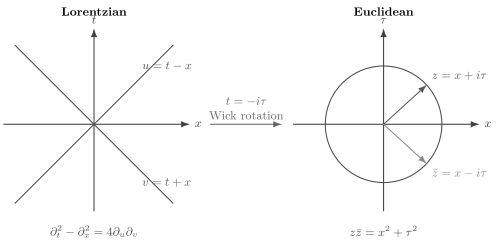
In Lorentzian signature, the massless wave operator separates along light-cone coordinates $u=t-x$ and $v=t+x$. After Wick rotation, the natural two-dimensional coordinates become $z=x+i\tau$ and $\bar z=x-i\tau$.

This is only a preview here. Later pages will use Euclidean continuation to turn oscillatory path integrals into statistical-mechanics weights and to define thermal field theory.

Nonrelativistic limit

For $m>0$ and $|\boldsymbol p|\ll m$,

$$\omega_{\boldsymbol p}=\sqrt{\boldsymbol p^2+m^2} =m+\frac{\boldsymbol p^2}{2m}-\frac{\boldsymbol p^4}{8m^3}+\cdots.$$

Therefore the normal-ordered relativistic free Hamiltonian becomes, at low momentum,

$$:H: =\int_{\boldsymbol p} \left(m+\frac{\boldsymbol p^2}{2m}+\cdots\right) a_{\boldsymbol p}^\dagger a_{\boldsymbol p}.$$

If particle number is fixed, the leading term is just $mN$, the total rest energy. Subtracting this constant leaves the nonrelativistic kinetic energy from the previous page. This is why nonrelativistic many-body theory is a low-energy shadow of relativistic field theory, not a completely separate language.

There is one important caveat. The free normal-ordered real scalar Hamiltonian commutes with the mode-counting operator $N=\int_{\boldsymbol p}a_{\boldsymbol p}^\dagger a_{\boldsymbol p}$, but this is not protected by a fundamental phase symmetry of a real field. Once interactions are added, a real scalar theory can create or destroy neutral quanta in combinations allowed by the interaction. To recover the nonrelativistic field $\psi$ with an exact number symmetry, one usually starts with a complex scalar field and isolates its slowly varying positive-frequency part. That is the natural topic of the next page.

Summary

The Klein–Gordon equation is the local relativistic wave equation for a scalar field. Its plane-wave solutions obey $p^2=m^2$, so each spatial momentum mode has frequency $\omega_{\boldsymbol p}=\sqrt{\boldsymbol p^2+m^2}$.

For $m>0$, the modes have positive oscillator frequencies, with the opposite-momentum coefficients related by the reality condition. Quantization uses $a_{\boldsymbol p}$ and $a_{\boldsymbol p}^\dagger$, with the field expansion arranged so that $[\phi(\boldsymbol x),\pi(\boldsymbol y)]=i\delta^{(3)}(\boldsymbol x-\boldsymbol y)$ as a continuum distributional identity.

The negative-frequency part of the real scalar field is not a negative-energy particle. It is the adjoint part of the field operator and creates positive-energy quanta. This is the first place where relativistic wave equations stop being single-particle equations and become equations for quantum fields.

Common pitfalls

The first trap is to interpret $\phi(x)$ as a probability wavefunction. In relativistic QFT, $\phi(x)$ is an operator-valued field. Its matrix elements can become wavefunctions in special limits, but the field itself is not a single-particle probability amplitude.

The second trap is to throw away the negative-frequency term. For a real quantum field, that term is required by hermiticity and by the equal-time commutation relations. Removing it destroys the local field.

The third trap is to lose a sign in the Klein–Gordon operator. With the mostly-minus metric used here, $\Box=\partial_t^2-\nabla^2$ and the free equation is $(\Box+m^2)\phi=0$.

The fourth trap is to confuse the zero-point energy with particle energy. With the finite regulator, the vacuum term $\frac12\sum_{\boldsymbol p}\omega_{\boldsymbol p}$ is a finite constant. The particle spectrum is measured relative to the selected vacuum by $:H:$; its continuum excitation operator is defined separately, not by subtracting an infinity.

The fifth trap is to mix oscillator-normalized and covariantly normalized states in one calculation. The field expansion with $1/\sqrt{2\omega_{\boldsymbol p}}$ pairs with $[a,a^\dagger]=(2\pi)^3\delta^{(3)}$; the invariant phase-space convention moves the same factor into the measure and the commutator.

Exercises

Exercise 1: derive the field equation from the action

Starting from

$$S=\int d^4x\,\left(\frac12\partial_\mu\phi\,\partial^\mu\phi-\frac12m^2\phi^2\right),$$

show that stationarity under smooth variations with compact support in the spacetime interior gives the interior equation

$$(\Box+m^2)\phi=0.$$

Solution

Vary $\phi\to\phi+\delta\phi$:

$$\delta S=\int d^4x\,\left(\partial_\mu\phi\,\partial^\mu\delta\phi-m^2\phi\,\delta\phi\right).$$

Integrating the first term by parts gives

$$\delta S=-\int d^4x\,\delta\phi\,(\partial_\mu\partial^\mu+m^2)\phi,$$

up to a boundary term. Since $\delta\phi$ is arbitrary, stationarity requires

$$(\Box+m^2)\phi=0.$$

Exercise 2: check the canonical commutator

Use the mode expansion

$$\phi(\boldsymbol x,t) =\int_{\boldsymbol p}\frac{1}{\sqrt{2\omega_{\boldsymbol p}}} \left(a_{\boldsymbol p}e^{-i\omega_{\boldsymbol p}t+i\boldsymbol p\cdot\boldsymbol x} +a_{\boldsymbol p}^\dagger e^{i\omega_{\boldsymbol p}t-i\boldsymbol p\cdot\boldsymbol x}\right)$$

and $[a_{\boldsymbol p},a_{\boldsymbol q}^\dagger]=(2\pi)^3\delta^{(3)}(\boldsymbol p-\boldsymbol q)$ to show that

$$[\phi(\boldsymbol x,t),\dot\phi(\boldsymbol y,t)]=i\delta^{(3)}(\boldsymbol x-\boldsymbol y).$$

Solution

Differentiate the field:

$$\dot\phi(\boldsymbol y,t) =\int_{\boldsymbol q}\left(-i\sqrt{\frac{\omega_{\boldsymbol q}}2}\right) \left(a_{\boldsymbol q}e^{-i\omega_{\boldsymbol q}t+i\boldsymbol q\cdot\boldsymbol y} -a_{\boldsymbol q}^\dagger e^{i\omega_{\boldsymbol q}t-i\boldsymbol q\cdot\boldsymbol y}\right).$$

Only the $a$–$a^\dagger$ commutators survive. At equal times,

$$\begin{aligned} [\phi(\boldsymbol x,t),\dot\phi(\boldsymbol y,t)] &=\frac{i}{2}\int_{\boldsymbol p} \left(e^{i\boldsymbol p\cdot(\boldsymbol x-\boldsymbol y)} +e^{-i\boldsymbol p\cdot(\boldsymbol x-\boldsymbol y)}\right) \\ &=i\int_{\boldsymbol p}e^{i\boldsymbol p\cdot(\boldsymbol x-\boldsymbol y)} \\ &=i\delta^{(3)}(\boldsymbol x-\boldsymbol y). \end{aligned}$$

In the second line, the two exponentials give the same integral after $\boldsymbol p\to-\boldsymbol p$ in one term.

Exercise 3: the low-momentum expansion

For $m>0$ and $|\boldsymbol p|\ll m$, show that

$$\sqrt{\boldsymbol p^2+m^2}=m+\frac{\boldsymbol p^2}{2m}+O(|\boldsymbol p|^4/m^3).$$

Explain why the leading term can be ignored in a fixed-particle-number nonrelativistic problem but not in a relativistic theory where particle number can change.

Solution

Write

$$\sqrt{\boldsymbol p^2+m^2}=m\sqrt{1+\frac{\boldsymbol p^2}{m^2}}.$$

Using $\sqrt{1+x}=1+x/2-x^2/8+\cdots$,

$$\sqrt{\boldsymbol p^2+m^2} =m+\frac{\boldsymbol p^2}{2m}-\frac{\boldsymbol p^4}{8m^3}+\cdots.$$

For fixed particle number $N$, the term $m$ contributes $mN$, a constant shift of all energies in that sector. If particle number can change, $mN$ is no longer a common constant across all states. It is the rest-energy cost of creating particles.

Exercise 4: massless solutions in one space dimension

For $m=0$ in one space dimension, solve

$$(\partial_t^2-\partial_x^2)\phi=0.$$

Solution

The operator factorizes:

$$\partial_t^2-\partial_x^2=(\partial_t-\partial_x)(\partial_t+\partial_x).$$

Introduce

$$u=t-x, \qquad v=t+x.$$

Then

$$\partial_t^2-\partial_x^2=4\partial_u\partial_v.$$

So the equation becomes

$$\partial_u\partial_v\phi=0.$$

Integrating once in $u$ and once in $v$ gives

$$\phi(u,v)=f(u)+g(v),$$

or

$$\phi(t,x)=f(t-x)+g(t+x).$$

These are right- and left-moving waves.

References and further reading

• Sidney Coleman, Lectures of Sidney Coleman on Quantum Field Theory, Chapter 3, for the construction of the scalar quantum field and the role of positive and negative frequencies.
• Mark Srednicki, Quantum Field Theory, Sections 1 and 3, for the relation between relativistic wave equations, scalar fields, and canonical quantization.
• Steven Weinberg, The Quantum Theory of Fields, Volume I, Chapters 5 and 7, for the particle-to-field logic and the canonical formalism.
• A. Zee, Quantum Field Theory in a Nutshell, Chapters I.3, I.4, and I.8, for physical motivation and canonical quantization of fields.