

Pole Residue and Wavefunction Renormalization
An isolated real pole in an exact two-point function tells us that the chosen field couples to a stable particle. Its residue tells us how strongly the field overlaps with that particle. This is more specific than the pole language of potential scattering on the previous page: poles of a -matrix can also describe bound states or, after continuation to another sheet, unstable resonances. LSZ uses the stable one-particle pole of a two-point function.
That distinction is easy to miss. In a free scalar theory the field is normalized so that its propagator has residue one at . In an interacting theory, the physical one-particle state is no longer the bare oscillator quantum. It is a dressed object: the field can create it, but it can also create multiparticle states with the same quantum numbers. The exact two-point function therefore contains an isolated one-particle pole plus a continuum. The coefficient of the isolated pole is the wavefunction renormalization factor .
This page develops the formula
and explains why
when the exact propagator is written in terms of a Lorentz-invariant self-energy . The same is the factor that appears on external legs in LSZ reduction. The next page turns this into the full scattering formula.
Three related quantities will appear, and keeping them separate prevents many normalization errors:
| Quantity | Meaning |
|---|---|
| residue of the covariant propagator as a function of | |
| residue of the positive-energy pole as a function of at fixed | |
| matrix element in covariant state normalization |
They are the same physical overlap viewed in three different variables.
The free pole and its residue
Section titled “The free pole and its residue”For a free real scalar field,
At fixed spatial momentum , define
Then
and the propagator decomposes as
The positive-energy pole is therefore at
with residue
Equivalently, in the Lorentz-invariant variable , the pole has residue :
Both statements are correct. The -residue contains an additional Jacobian because
near the positive-energy pole.
The time-domain propagator makes the physical meaning especially clear. For ,
The pole gives a long-lived oscillation. In an interacting theory, the exact one-particle pole gives the same kind of oscillation, but with shifted frequency and changed amplitude.
Exact propagator and the physical pole
Section titled “Exact propagator and the physical pole”The exact propagator is obtained by summing all 1PI self-energy insertions:
A stable scalar particle of physical mass appears as an isolated zero of the exact inverse propagator:
Thus
This equation is implicit. The self-energy must be evaluated at the physical pole, not at the bare mass unless one is working only to the lowest nontrivial order.
To find the residue, expand the inverse propagator around :
Since ,
Therefore
The pole residue is
So near the physical pole,
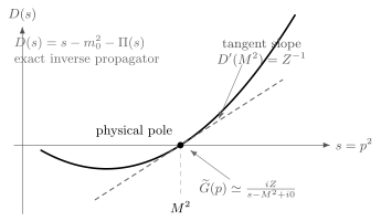
The physical mass is the zero of the exact inverse propagator . The slope at the zero is , so the propagator has residue .
The mass shift and the residue are different effects. The value of at the pole moves the pole; the derivative of at the pole changes the normalization of the pole. Constant self-energy insertions renormalize the mass but do not produce wavefunction renormalization. Momentum-dependent self-energy insertions produce both.
In perturbation theory one often expands around the bare mass, but the clean definition is the pole definition above. The residue must be evaluated at , not merely at , unless the difference is beyond the order being computed.
Residue as field–particle overlap
Section titled “Residue as field–particle overlap”The exact propagator also has a nonperturbative interpretation. Insert a complete set of exact energy-momentum eigenstates between the two fields. For ,
contains terms of the form
with the appropriate normalization of states. If there is a stable one-particle state of mass , its energy is
Choose the one-particle state phase so that the nonzero overlap is positive, and define by
in the standard relativistic normalization
Then the one-particle part of the exact two-point function is
which Fourier transforms to
Thus measures the amplitude squared for the field to create the physical one-particle state from the vacuum. A badly chosen field may have a small overlap with the particle even though the particle is present in the spectrum. A field with the wrong quantum numbers has for that particle.
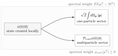
A local field acting on the vacuum does not create only a single bare quantum. In an interacting theory it creates the physical one-particle sector with amplitude , together with continuum states carrying the same quantum numbers. In the diagram, is the invariant one-particle measure and projects onto the multiparticle continuum.
This explains the historical phrase “wavefunction renormalization.” The word is slightly misleading in relativistic QFT: we are not renormalizing a Schrödinger wavefunction. We are renormalizing the normalization of the field operator relative to the physical one-particle state.
Spectral representation and the bound on Z
Section titled “Spectral representation and the bound on Z”The exact two-point function admits the Källén–Lehmann representation
where is a positive spectral density in a unitary theory with positive-norm states. If the lightest state created by is a stable particle of mass , the spectral density contains a delta function. For clarity, assume here that it is the only isolated stable state below the first continuum threshold:
Therefore
Here is the multiparticle threshold in the same quantum-number channel. The first term is the isolated particle pole. The integral is the branch cut associated with multiparticle states.
If several stable particles with the same quantum numbers lie below the continuum, the first term is replaced by in , and the propagator contains one isolated pole for each such state. Nothing in the LSZ argument changes: each asymptotic species is reduced at its own pole.
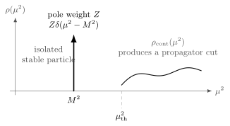
In the single-pole case shown, the exact spectral density splits into an isolated one-particle contribution and a continuum beginning at the first multiparticle threshold . The pole and the cut are two pieces of the same exact two-point function.
The pole and continuum also have sharply different late-time behavior. The isolated pole gives a persistent oscillation. A continuum contribution dephases and is controlled asymptotically by its threshold singularity. For example, suppose the physical discontinuity has the near-threshold behavior
Its large-time contribution then has the characteristic form
up to a convention-dependent complex coefficient. Thus a branch point produces a power-law tail, whereas an isolated stable pole produces an undamped one-particle oscillation.
For a canonically normalized scalar field, the equal-time commutation relation implies the spectral sum rule
Since ,
This inequality is a statement about the spectral weight of the bare canonical field. It is not a universal statement about every possible rescaled field. If we define a renormalized field
then has unit one-particle overlap by construction, and its propagator has unit residue at the pole.
There is also an important limitation: if the would-be particle is unstable, the pole moves off the physical real axis onto a different sheet. Then there is no normalizable asymptotic one-particle state and no positive real with the same direct probability interpretation. Resonance residues are still meaningful, but they are analytic-continuation data rather than probabilities.
This distinction is important in phenomenology. Stable external particles belong in the LSZ formula. Unstable resonances appear as internal structures in amplitudes and are described by pole positions and residues after analytic continuation.
General energy-dependent self-energy
Section titled “General energy-dependent self-energy”The Lorentz-invariant formula assumes that the vacuum is Lorentz invariant and that the self-energy depends only on . In some settings, especially nonrelativistic systems or finite-density media, the denominator is more naturally written as
The dispersion relation is determined by
Near the positive-energy pole,
Therefore
The residue in the plane is
If , then
and the fixed- residue becomes
This is the same as the covariant pole residue. The extra is just the conversion from the variable to the variable .
External poles of n-point functions
Section titled “External poles of n-point functions”The reason matters for scattering is that an -point Green function has one exact propagator attached to each external field insertion. Near the simultaneous external one-particle poles, the connected momentum-space Green function has the schematic form
where are the arguments of the forward transform with phase . For future-directed physical momenta , use on an incoming leg and on an outgoing leg. The next lesson derives this assignment from the external mode overlaps.
This formula packages two facts. First, each field insertion creates or annihilates a physical particle with amplitude . Second, once the external propagation has been stripped away, the remaining object is the scattering amplitude .
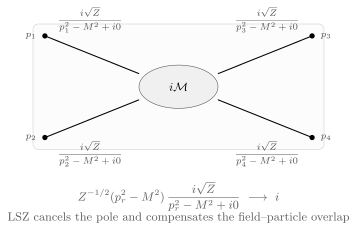
Near the one-particle poles, an exact Green function factorizes into external pole factors and the physical amplitude , with the overall momentum delta suppressed. The labels are physical momenta. The displayed operation leaves one per leg; the complete LSZ amputator also divides by that .
This is the bridge to LSZ reduction. On either plane-wave phase,
Thus the complete coordinate operator becomes the momentum-space amputator . It cancels both the pole and its numerator . The corresponding unit-residue factor appears in Tong, HTML edition 2021, § 3.7.2, reduction formula following Eq. (3.306). If instead we use , the pole residue is one and the overlap factors are already absorbed into the field. The stable-state LSZ treatment explains the external-state hypotheses and the distinction from full-propagator amputation.
Example: a momentum-dependent self-energy
Section titled “Example: a momentum-dependent self-energy”Suppose the self-energy near the pole can be approximated by
where and are perturbatively small. The exact inverse propagator is
The pole equation gives
so
The residue is
The constant part shifts the mass. The coefficient changes the residue. This is why a momentum-independent tadpole in theory contributes to mass renormalization but not to wavefunction renormalization at that order.
For the exact propagator of a canonically normalized scalar field, spectral positivity gives . In the present sign convention this implies when the linear approximation is evaluated at the pole. The algebraic toy parametrization itself does not impose that inequality unless it is required to represent such a unitary canonical two-point function.
Summary
Section titled “Summary”An interacting scalar two-point function contains more information than the position of its pole. The physical mass is defined by the zero of the exact inverse propagator,
while the pole residue is
The same has a spectral interpretation:
so it measures the overlap of the chosen field with the physical one-particle state. In the Källén–Lehmann representation, the exact propagator is an isolated pole plus a continuum. For a canonically normalized scalar field in a positive-norm Hilbert space, the spectral sum rule gives .
For scattering, the important consequence is factorization near external poles. Each external field insertion supplies a pole and a factor . LSZ reduction removes the external poles and converts Green functions into -matrix elements with the correct field-normalization factors.
Common pitfalls
Section titled “Common pitfalls”- The pole location and pole residue are not the same datum. fixes the mass shift; fixes .
- The inequality assumes a canonically normalized field and a positive Hilbert-space metric. It is not a statement about an arbitrarily rescaled field.
- A momentum-independent self-energy can renormalize the mass without renormalizing the field.
- The -plane residue and the covariant residue differ by a factor .
- An unstable resonance does not have the same LSZ external-particle interpretation as a stable particle. Its pole is off the physical real axis.
- External legs in LSZ must use the physical mass , not the bare mass parameter .
- The symbol can mean either the pole residue or a field-strength counterterm depending on context. In this page it is the physical pole residue of the chosen field.
Exercises
Section titled “Exercises”Exercise 1
Section titled “Exercise 1”Let
Assume a stable pole at . Derive the pole residue .
Solution
Write
The pole mass obeys
Expanding around ,
The first term vanishes, and
Therefore
with
Exercise 2
Section titled “Exercise 2”Use the Källén–Lehmann form
and the canonical sum rule
to show that when the spectral density contains
Solution
Substitute the decomposition into the sum rule:
This gives
In a positive-norm Hilbert space, the spectral density is nonnegative:
Hence
Also the isolated pole weight itself is nonnegative, so
Therefore
Exercise 3
Section titled “Exercise 3”At fixed , suppose an exact propagator has a stable pole
Compute the large-positive-time contribution to
Solution
For , close the contour in the lower half-plane. The positive-energy Feynman pole lies at
Using
only the first pole contributes for . Therefore
The continuum contributes additional oscillatory integrals beginning at threshold. At very large , the isolated pole gives the clean one-particle oscillation, while the continuum gives threshold-suppressed or branch-cut contributions.
Exercise 4
Section titled “Exercise 4”Let a four-point connected Green function near its external poles behave as
Here for incoming/outgoing physical momenta as above, so . Show what remains after applying one factor of to each external leg, keeping the overall phase.
Solution
Apply
to the pole form. The factor on each leg gives
as the on-shell limit is taken. The four factors give , so the central factor of remains:
This is the connected -matrix element. Dividing out its explicit and momentum delta gives . Using the complete amputator instead leaves unity on each leg and reaches the same result for four legs; retaining that per-leg is necessary for a general number of external particles.
References
Section titled “References”- Tong, David. Quantum Field Theory. University of Cambridge lecture notes, HTML edition, 2021. § 3.7.2, “From Green’s Functions to S-Matrices”.
Further reading
Section titled “Further reading”- Sidney Coleman, Lectures on Quantum Field Theory, edited by Bryan Gin-ge Chen et al., World Scientific, 2019, chapters 14–15.
- H. Lehmann, “On the Properties of Propagation Functions and Renormalization Constants of Quantized Fields,” Il Nuovo Cimento 11 (1954), 342–357.
- H. Lehmann, K. Symanzik, and W. Zimmermann, “On the Formulation of Quantized Field Theories,” Il Nuovo Cimento 1 (1955), 205–225.
- Mark Srednicki, Quantum Field Theory, Cambridge University Press, 2007, sections 13–14 and 27.
- K. Symanzik, “On the Many-Particle Structure of Green’s Functions in Quantum Field Theory,” Journal of Mathematical Physics 1 (1960), 249–273.
- Steven Weinberg, The Quantum Theory of Fields, Volume I: Foundations, Cambridge University Press, 1995, sections 10.3 and 10.7.
- A. Zee, Quantum Field Theory in a Nutshell, 2nd edition, Princeton University Press, 2010, chapter III.3.
Original QFT.org content:CC BY 4.0, unless an item supplies different terms. Third-party material retains its own terms.