Pole Shifts, Mass Renormalization, and 1PI Diagrams

The previous page reorganized the exact two-point function as a free propagator dressed by all possible one-particle-irreducible self-energy insertions. The algebra looked almost too simple: a geometric series of insertions became a shift of the inverse propagator. The real content of that shift is physical. It tells us that the mass appearing in the free Lagrangian is not automatically the mass of the observed particle.

A particle in an interacting theory is recognized by a pole of an exact Green function. The pole position gives the physical mass; the residue tells how strongly the field creates that particle from the vacuum; the remaining singularities describe multiparticle states. This page explains the first of these statements in detail. It is the point where the formal Dyson equation becomes the practical language of mass renormalization.

The discussion below assumes a stable scalar particle unless stated otherwise. For an unstable particle the pole moves off the real axis on the appropriate unphysical sheet; then the real and imaginary parts of the pole encode the mass and width rather than a single real mass-shell equation.

Poles define physical masses

Physical-pole self-energy sign

This page continues the self-energy convention

$$\Delta(p)=\frac{i}{p^2-m^2-\Pi(p^2)+i\epsilon}.$$

With this convention, a stable physical pole at $p^2=M^2$ satisfies

$$M^2-m^2-\operatorname{Re}\Pi(M^2)=0.$$

Authors often differ by signs or factors of $i$ in the definition of the self-energy. The invariant statement is the location of the zero of the exact inverse propagator.

For a free scalar field, the momentum-space propagator is

$$\Delta_0(p)=\frac{i}{p^2-m^2+i\epsilon}.$$

The denominator vanishes at

$$p^2=m^2.$$

This is not merely an algebraic accident. The pole is the Green-function signature of a one-particle state with relativistic dispersion relation

$$p^0=\omega_{\mathbf p}=\sqrt{\mathbf p^2+m^2}.$$

In an interacting theory, the exact propagator takes the Dyson-resummed form

$$\Delta(p)=\frac{i}{D(p^2)+i\epsilon}, \qquad D(s)=s-m^2-\Pi(s), \qquad s=p^2.$$

A stable scalar particle of mass $M$ appears as an isolated zero of $D(s)$:

$$D(M^2)=0.$$

Equivalently,

$$\boxed{M^2=m^2+\operatorname{Re}\Pi(M^2).}$$

This equation is implicit because the self-energy is evaluated at the physical pole, not at an arbitrary external momentum. If the interaction is weak, we can solve it perturbatively. Suppose

$$\Pi(s)=\lambda \Pi_1(s)+\lambda^2\Pi_2(s)+O(\lambda^3),$$

and write

$$M^2=m^2+\lambda a_1+\lambda^2 a_2+O(\lambda^3).$$

Substituting into $M^2-m^2-\Pi(M^2)=0$ gives

$$\lambda a_1+\lambda^2 a_2 = \lambda \Pi_1(m^2+\lambda a_1+\cdots) +\lambda^2\Pi_2(m^2+\cdots)+O(\lambda^3).$$

Expanding the first term about $s=m^2$,

$$\Pi_1(m^2+\lambda a_1+\cdots) = \Pi_1(m^2)+\lambda a_1\Pi_1'(m^2)+O(\lambda^2).$$

Therefore

$$a_1=\Pi_1(m^2), \qquad a_2=\Pi_2(m^2)+\Pi_1(m^2)\Pi_1'(m^2).$$

To first order, the mass-squared shift is simply

$$\delta M^2=\lambda\Pi_1(m^2)+O(\lambda^2),$$

but beyond leading order the momentum dependence of the self-energy matters.

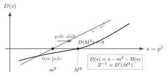
The free pole sits at the zero of $s-m^2$. Interactions replace the inverse propagator by $D(s)=s-m^2-\Pi(s)$, and the physical pole moves to the zero $D(M^2)=0$. Near that zero the slope fixes the pole residue.

Near the physical pole,

$$D(s)=D'(M^2)(s-M^2)+O((s-M^2)^2),$$

so

$$\Delta(p)\simeq \frac{iZ}{p^2-M^2+i\epsilon}, \qquad Z=\frac{1}{1-\Pi'(M^2)}.$$

The residue $Z$ will become central later, especially in LSZ reduction. For now the important point is that the pole location and the residue are separate pieces of information: the first defines the particle mass, while the second measures the overlap between the field $\phi$ and the physical one-particle state.

A 0+1-dimensional warm-up: the anharmonic oscillator

A useful way to see pole shifts without the complications of momentum integrals is to study a single oscillator with interaction

$$H=H_0+V, \qquad H_0=\frac12\pi^2+\frac12m^2q^2, \qquad V=\frac{\lambda}{4!}q^4.$$

This is field theory in $0+1$ dimensions: time exists, but there is no spatial momentum. It is therefore a cleaner warm-up than a full relativistic field theory: poles are ordinary energy gaps, and multiparticle continua are replaced by discrete higher oscillator levels. The free two-point function is

$$G_0(t)=\langle 0|Tq(t)q(0)|0\rangle =\frac{1}{2m}e^{-im|t|},$$

and its Fourier transform has poles at $\omega=\pm m$:

$$G_0(\omega)=\frac{i}{\omega^2-m^2+i\epsilon}.$$

The exact time-ordered two-point function has a spectral expansion. If $|\Omega\rangle$ is the true ground state and $|n\rangle$ are exact energy eigenstates, then schematically

$$G(\omega) = i\sum_n \frac{2(E_n-E_\Omega)|\langle \Omega|q|n\rangle|^2} {\omega^2-(E_n-E_\Omega)^2+i\epsilon}.$$

Only states with the right parity and quantum numbers appear. In the free oscillator, $q$ connects $|0\rangle$ only to the one-quantum state $|1\rangle$, so the only positive-energy pole is at $\omega=m$. In the anharmonic oscillator, the exact eigenstates are mixtures of the free oscillator levels, and the pole moves from $m$ to

$$M=E_1-E_\Omega.$$

The pole shift is therefore just ordinary perturbation theory written in Green-function language. This is the conceptual bridge: in a field theory, a mass is an energy gap at zero spatial momentum, extended by Lorentz invariance to the full mass shell.

As a quick check, first-order time-independent perturbation theory gives

$$\delta E_n=\frac{\lambda}{4!}\langle n|q^4|n\rangle.$$

Using

$$q=\frac{a+a^\dagger}{\sqrt{2m}},$$

one finds

$$\langle n|q^4|n\rangle =\frac{6n^2+6n+3}{4m^2}.$$

Thus

$$\delta E_n=\frac{\lambda}{32m^2}(2n^2+2n+1).$$

The first excitation energy shifts by

$$\delta(E_1-E_0)=\frac{\lambda}{8m^2}.$$

This is the simplest possible version of mass renormalization: an interaction changes the energy gap, and the Green-function pole follows that change.

Intermediate states and the origin of extra denominators

Perturbative self-energies do more than shift a number. They reveal which virtual intermediate states the field can fluctuate into.

In the anharmonic oscillator with $q^4$ interaction, a two-vertex self-energy diagram can contain an intermediate state with three free quanta. In frequency space this produces a denominator of the form

$$\Pi_{3}(\omega^2) \sim \frac{C\lambda^2}{\omega^2-(3m)^2+i\epsilon},$$

where $C$ is a positive constant depending on normalization and vertex conventions. The corresponding pole equation is

$$\omega^2=m^2+\frac{C\lambda^2}{\omega^2-9m^2+i\epsilon}+\cdots.$$

Near the one-particle pole, $\omega^2\approx m^2$, so

$$\omega^2 \approx m^2-\frac{C\lambda^2}{8m^2}+\cdots.$$

The sign comes from evaluating the intermediate-state denominator below the three-particle energy. The same expression also warns us that perturbation theory knows about other singularities. It is not only correcting the one-particle pole; it is also sensing the states near $\omega=3m$.

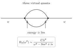
A two-vertex self-energy in the oscillator can send a one-quantum state into a virtual three-quantum state and back. This is the origin of denominators such as $\omega^2-9m^2+i\epsilon$ in the self-energy.

In ordinary field theory, the same idea becomes richer because intermediate particles can carry continuous momenta. A discrete denominator is replaced by an integral. For example, a multiparticle contribution may contain

$$\int \frac{d^3k_1}{(2\pi)^3 2\omega_{\mathbf k_1}} \frac{d^3k_2}{(2\pi)^3 2\omega_{\mathbf k_2}} \cdots \frac{1}{p^0-\omega_{\mathbf k_1}-\omega_{\mathbf k_2}-\cdots+i\epsilon}.$$

The denominator can vanish when the external energy reaches the energy of real multiparticle states. In $0+1$ dimensions this gives additional poles. In field theory it usually gives branch cuts beginning at thresholds such as $p^2=4M^2$ or $p^2=9M^2$. Those thresholds are the subject of the later discussion of spectral representations and cuts.

Mass renormalization as a choice of parameters

The phrase mass renormalization has two closely related meanings. First, it names the physical phenomenon: interactions shift the pole of the propagator. Second, it names the calculational prescription: we introduce a renormalized mass and compensating counterterms, then fix that mass by a stated renormalization condition. Only in an on-shell scheme is the mass parameter used in perturbation theory chosen to equal the physical pole mass. In schemes such as $\overline{\rm MS}$, the renormalized mass depends on the subtraction scale, and the pole mass is a derived quantity.

Start with a bare scalar theory,

$$\mathcal L = \frac12\partial_\mu\phi_0\partial^\mu\phi_0 -\frac12m_0^2\phi_0^2 -\frac{\lambda_0}{4!}\phi_0^4.$$

The bare parameters $m_0$ and $\lambda_0$ are not directly measured. To illustrate the on-shell choice, write the theory in terms of the physical mass $M$ and compensating counterterms:

$$\mathcal L = \frac12\partial_\mu\phi\partial^\mu\phi -\frac12M^2\phi^2 -\frac{\lambda}{4!}\phi^4 +\mathcal L_{\mathrm{ct}},$$

with

$$\mathcal L_{\mathrm{ct}} = \frac12\delta Z\,\partial_\mu\phi\partial^\mu\phi -\frac12\delta m^2\phi^2 -\frac{\delta\lambda}{4!}\phi^4+\cdots.$$

The ellipsis reminds us that the set of needed counterterms depends on the theory and the order of perturbation theory. For the two-point function, it is convenient to package the loop and counterterm contributions as

$$\Pi_{\mathrm{ren}}(s) = \Pi_{\mathrm{loop}}(s)+\Pi_{\mathrm{ct}}(s), \qquad s=p^2.$$

In an on-shell scheme for a stable particle, after choosing the renormalized mass parameter in the quadratic Lagrangian to be the physical mass $M$, we impose

$$\operatorname{Re}\Pi_{\mathrm{ren}}(M^2)=0, \qquad \operatorname{Re}\Pi_{\mathrm{ren}}'(M^2)=0.$$

The first condition says that loop corrections plus counterterms do not move the pole away from $p^2=M^2$. The second says that the residue of the renormalized propagator is normalized to one. This is a convention for the field normalization, not an extra physical measurement. When LSZ reduction is introduced, this second condition will be recognized as a convenient way of removing external-leg residue factors from the final scattering rules.

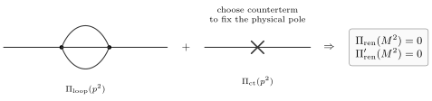
A mass counterterm is chosen together with the loop self-energy so that the renormalized inverse propagator has its zero at the physical mass. In an on-shell scheme the loop shift and the counterterm cancel at $p^2=M^2$.

This is not a trick for hiding physics. It is a separation between what is measured and what is calculated. If $M$ is the observed mass, then perturbation theory should be organized around particles of mass $M$, not around an unobservable bare mass that changes when the cutoff or subtraction convention changes.

Why 1PI diagrams are the right building blocks

A connected two-point diagram may contain a chain of self-energy insertions joined by ordinary propagators. Such a diagram is connected, but it is not elementary. Cutting a single internal line can split it into two pieces. This is why the exact two-point function is not built from all connected two-point diagrams as primitive objects; it is built from 1PI self-energy blocks.

For the propagator,

$$\Delta= \Delta_0+ \Delta_0(-i\Pi)\Delta_0 +\Delta_0(-i\Pi)\Delta_0(-i\Pi)\Delta_0+\cdots.$$

The self-energy $\Pi$ itself contains only 1PI two-point diagrams. If we allowed one-particle-reducible diagrams inside $\Pi$, the Dyson series would count the same chain multiple times.

The same logic generalizes. An $n$-point 1PI diagram is a connected diagram that cannot be disconnected by cutting one internal line. These diagrams are also called proper vertices. In a more advanced language, the collection of all 1PI functions is generated by the quantum effective action $\Gamma[\phi]$. The second functional derivative of $\Gamma$ gives the exact inverse propagator, while higher derivatives give exact interaction vertices.

For this course, the key practical rule is simpler:

$$\text{full connected diagrams} = \text{propagators glued together by 1PI kernels}.$$

This is the diagrammatic reason why pole shifts are read from the 1PI self-energy and not from an arbitrary connected two-point graph.

From the oscillator back to relativistic fields

The oscillator discussion has no spatial momentum. A relativistic scalar field has one oscillator for every momentum mode. With the common noncovariant oscillator normalization $[a_{\mathbf p},a^\dagger_{\mathbf q}]=(2\pi)^3\delta^{(3)}(\mathbf p-\mathbf q)$, a free scalar field of physical mass $M$ has

$$H_0=\int \frac{d^3p}{(2\pi)^3}\,\omega_{\mathbf p}\, a^\dagger_{\mathbf p}a_{\mathbf p}, \qquad \omega_{\mathbf p}=\sqrt{\mathbf p^2+M^2},$$

and

$$\phi(x) = \int\frac{d^3p}{(2\pi)^3}\frac{1}{\sqrt{2\omega_{\mathbf p}}} \left( a_{\mathbf p}e^{-ip\cdot x} +a^\dagger_{\mathbf p}e^{ip\cdot x} \right), \qquad p^0=\omega_{\mathbf p}.$$

This is equivalent to the qft.org covariant normalization used in the conventions page; the factors of $2\omega_{\mathbf p}$ have simply been moved from the measure into the operators. The pole statements below are independent of this bookkeeping choice.

Interactions couple these infinitely many oscillators. The exact propagator still has poles, but now the pole condition is Lorentz invariant:

$$p^2=M^2.$$

The pole in $p^0$ at fixed $\mathbf p$ occurs at

$$p^0=\sqrt{\mathbf p^2+M^2}.$$

Thus mass renormalization is not merely an energy shift at zero momentum. It shifts the entire mass shell. Lorentz invariance ensures that the same $M$ appears for every $\mathbf p$.

Composite operators and multiparticle singularities

The field $\phi$ is designed to have overlap with the one-particle state. Other operators create other collections of states. For example, a renormalized composite operator $[\phi^2]_R$ has the quantum numbers of two scalar particles. Its connected two-point function

$$C_2(x-y)=\langle\Omega|T[\phi^2]_R(x)[\phi^2]_R(y)|\Omega\rangle_c$$

contains two-particle singularities. The subscript $c$ removes the vacuum-disconnected constant. The label $R$ matters because products of fields at one point require their own ultraviolet renormalization and can mix with other local operators; these local subtractions do not remove the physical threshold. In a free oscillator, the vacuum-subtracted operator $q^2-\langle q^2\rangle$ connects the ground state to a two-quantum state, so the Fourier transform has a pole near

$$\omega=2m.$$

In a relativistic field theory, $[\phi^2]_R$ creates two-particle states with arbitrary relative momentum. The corresponding singularity is not usually a single pole but a branch cut beginning at

$$p^2=(2M)^2.$$

This distinction is important. A simple isolated pole signals a stable one-particle state. A continuum of multiparticle states produces a cut. Bound states, if present, appear as additional poles below the multiparticle threshold. The analytic structure of Green functions is therefore a map of the spectrum.

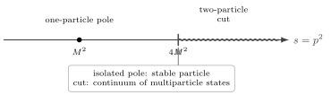
A field with overlap onto a stable particle produces an isolated pole at $p^2=M^2$. Composite operators and virtual intermediate states also reveal multiparticle thresholds, such as $p^2=4M^2$ for two identical scalar particles.

The next pages develop this point systematically: commutators constrain causal support, spectral representations encode positivity and thresholds, and scattering amplitudes are extracted from the pole structure of exact Green functions.

Summary

The exact propagator is not just a dressed version of the free propagator. It is a spectral diagnostic. Its isolated poles identify stable particles, and their positions define physical masses. In the self-energy convention used here,

$$\Delta(p)=\frac{i}{p^2-m^2-\Pi(p^2)+i\epsilon},$$

so the physical mass satisfies

$$M^2-m^2-\operatorname{Re}\Pi(M^2)=0.$$

Perturbatively, self-energy diagrams shift the pole. A counterterm can then be chosen so that the pole is placed at the measured mass. This is mass renormalization: the interaction really changes the relation between bare parameters and physical observables, and the counterterm organizes perturbation theory around the physical observable.

The 1PI condition is the diagrammatic mechanism behind this organization. A self-energy is a one-particle-irreducible two-point kernel. The full propagator is obtained by gluing such kernels together with ordinary propagators. This avoids overcounting and turns the infinite chain of insertions into the compact Dyson denominator.

Common pitfalls

• The mass in the Lagrangian is not automatically the physical mass. It becomes the physical mass only after a renormalization condition has been imposed.
• The pole equation is nonlinear: for a stable particle $M^2=m^2+\operatorname{Re}\Pi(M^2)$, not $M^2=m^2+\Pi(0)$ or $m^2+\Pi(m^2)$ except at leading order.
• A connected two-point diagram is not necessarily a self-energy. The self-energy contains only 1PI two-point diagrams.
• A virtual intermediate state in a self-energy is not a real decay unless the external momentum reaches the corresponding physical threshold.
• A counterterm is not an optional patch. It is part of the definition of which physical parameters are held fixed in perturbation theory.

Exercises

Exercise 1: perturbative pole location

Let

$$\Delta(s)=\frac{i}{s-m^2-\Pi(s)+i\epsilon}, \qquad \Pi(s)=\lambda A+\lambda^2(B+C(s-m^2))+O(\lambda^3),$$

where $A$, $B$, and $C$ are constants. Find the physical pole $M^2$ through order $\lambda^2$.

Solution

Write

$$M^2=m^2+\lambda a_1+\lambda^2a_2+O(\lambda^3).$$

The pole condition is

$$M^2-m^2-\Pi(M^2)=0.$$

Now

$$\Pi(M^2) = \lambda A+ \lambda^2\left(B+C(M^2-m^2)\right)+O(\lambda^3).$$

Since $M^2-m^2=O(\lambda)$, the term $\lambda^2 C(M^2-m^2)$ is actually $O(\lambda^3)$ and does not contribute through order $\lambda^2$. Therefore

$$\lambda a_1+\lambda^2a_2 = \lambda A+\lambda^2B+O(\lambda^3),$$

so

$$\boxed{M^2=m^2+\lambda A+\lambda^2B+O(\lambda^3).}$$

The derivative term $C$ first affects the pole position at order $\lambda^3$ in this particular parametrization, but it affects the residue already at order $\lambda^2$.

Exercise 2: residue of a dressed pole

For

$$\Delta(s)=\frac{i}{s-m^2-\Pi(s)+i\epsilon},$$

assume there is a stable pole at $s=M^2$. Show that the pole residue is

$$Z=\frac{1}{1-\Pi'(M^2)}.$$

Solution

Define

$$D(s)=s-m^2-\Pi(s).$$

The pole condition is $D(M^2)=0$. Expanding around $M^2$,

$$D(s)=D(M^2)+D'(M^2)(s-M^2)+O((s-M^2)^2).$$

Since $D(M^2)=0$ and

$$D'(s)=1-\Pi'(s),$$

we have

$$D(s)=\left(1-\Pi'(M^2)\right)(s-M^2)+\cdots.$$

Therefore

$$\Delta(s) \simeq \frac{i}{(1-\Pi'(M^2))(s-M^2)+i\epsilon} = \frac{iZ}{s-M^2+i\epsilon},$$

with

$$\boxed{Z=\frac{1}{1-\Pi'(M^2)}}.$$

The placement of $i\epsilon$ in the last expression is shorthand for the corresponding pole prescription near the physical pole.

Exercise 3: first-order mass shift in the quartic oscillator

For

$$H_0=\frac12\pi^2+\frac12m^2q^2, \qquad V=\frac{\lambda}{4!}q^4,$$

use

$$q=\frac{a+a^\dagger}{\sqrt{2m}}$$

to show that the first excitation energy shifts by

$$\delta(E_1-E_0)=\frac{\lambda}{8m^2}.$$

Solution

The first-order energy shift is

$$\delta E_n=\langle n|V|n\rangle =\frac{\lambda}{4!}\langle n|q^4|n\rangle.$$

Using the oscillator algebra, one may normal-order $(a+a^\dagger)^4$ or evaluate it directly. The standard result is

$$\langle n|(a+a^\dagger)^4|n\rangle=6n^2+6n+3.$$

Since $q=(a+a^\dagger)/\sqrt{2m}$,

$$\langle n|q^4|n\rangle =\frac{6n^2+6n+3}{4m^2}.$$

Thus

$$\delta E_n =\frac{\lambda}{24}\frac{6n^2+6n+3}{4m^2} =\frac{\lambda}{32m^2}(2n^2+2n+1).$$

For $n=1$,

$$\delta E_1=\frac{5\lambda}{32m^2},$$

while for $n=0$,

$$\delta E_0=\frac{\lambda}{32m^2}.$$

Therefore

$$\boxed{\delta(E_1-E_0)=\delta E_1-\delta E_0=\frac{\lambda}{8m^2}.}$$

This shift is the oscillator analogue of the shift of a particle pole in the two-point function.

References and further reading

• Sidney Coleman, Lectures on Quantum Field Theory, Chapter 10, for a detailed discussion of mass renormalization, counterterms, and the transition from Wick diagrams to Feynman diagrams.
• Mark Srednicki, Quantum Field Theory, Sections 13–15, for the exact propagator, the Källén–Lehmann representation, and loop corrections to propagators.
• Steven Weinberg, The Quantum Theory of Fields, Volume I, Sections 10.3 and 10.7, for field and mass renormalization, pole residues, and spectral representations.
• A. Zee, Quantum Field Theory in a Nutshell, Part III, Chapter III.3, for the distinction between bare and physical perturbation theory.

References

Section titled “References”- Schwartz, Matthew D. Quantum Field Theory and the Standard Model. Cambridge University Press, 2014, first printing. DOI: 10.1017/9781139540940.
- Srednicki, Mark. Quantum Field Theory. Author prepublication draft, 2006. Author’s source page. Open PDF.
Further reading
Section titled “Further reading”- Coleman, Sidney. Lectures of Sidney Coleman on Quantum Field Theory. Edited by Bryan Gin-ge Chen, David Derbes, David Griffiths, Brian Hill, Richard Sohn, and Yuan-Sen Ting; foreword by David Kaiser. Singapore: World Scientific, 2019. DOI: 10.1142/9371. Chapter 10, “Mass renormalization and Feynman diagrams.”
- Weinberg, Steven. The Quantum Theory of Fields, Volume I: Foundations. Cambridge University Press, 1995. DOI: 10.1017/CBO9781139644167.
- Zee, A. Quantum Field Theory in a Nutshell. 2nd ed. Princeton, NJ: Princeton University Press, 2010. Publisher. Part III, Chapter III.3, “Counterterms and Physical Perturbation Theory.”
Original QFT.org content:CC BY 4.0, unless an item supplies different terms. Third-party material retains its own terms.