LSZ Reduction and Cross Sections

The preceding lesson explained how an interacting scalar field remembers physical particles: an exact two-point function has an isolated pole at the physical mass, and the residue of that pole is the wavefunction factor $Z$. This page turns that pole statement into observable physics.

There are two separate operations. First, LSZ reduction strips the external one-particle poles from time-ordered Green functions, leaving a finite on-shell scattering amplitude. Second, phase-space kinematics converts the squared amplitude into a transition rate, decay width, or cross section. The first step is field theory; the second step is relativistic probability bookkeeping.

This is the point where diagrams stop being merely a way to compute correlation functions and become a way to compute things measured in scattering experiments.

The nonrelativistic warm-up

Covariant states and physical momenta

One-particle states are covariantly normalized as

$$\langle \mathbf p|\mathbf q\rangle =(2\pi)^3 2E_{\mathbf p}\,\delta^{(3)}(\mathbf p-\mathbf q), \qquad E_{\mathbf p}=\sqrt{\mathbf p^2+M^2}.$$

The invariant on-shell measure is

$$d\Pi(p)={d^3\mathbf p\over (2\pi)^3 2E_{\mathbf p}}.$$

The connected S-matrix element is defined by

$$\langle f|S|i\rangle_{\mathrm{conn}} =i(2\pi)^4\delta^{(4)}(P_f-P_i)\,\mathcal M_{i\to f}.$$

Throughout, $p_j$ denotes a future-directed physical momentum. The Fourier arguments $q_j$ of a Green function are separate variables. With the forward phase $e^{+i\sum_jq_j\cdot x_j}$ used below, incoming legs have $q=-p$ and outgoing legs have $q=+p$. The external mode overlaps determine these signs; a momentum arrow labeled $p$ in a scattering diagram still denotes the physical momentum.

With other common conventions, factors of $i$ may move between $\mathcal M$, the amputated vertex, and the Feynman rules. Cross sections depend on $|\mathcal M|^2$ and are convention-independent.

Before discussing LSZ, it is useful to recall the familiar potential-scattering formula. For a nonrelativistic particle with free Hamiltonian $H_0$ and interaction $V$, the resolvent has the Born expansion

$$G(E)={1\over E-H+i0} =G_0(E)+G_0(E)VG_0(E)+G_0(E)VG_0(E)VG_0(E)+\cdots,$$

where

$$G_0(E)={1\over E-H_0+i0}.$$

The corresponding transition matrix is

$$T(E)=V+VG_0(E)V+VG_0(E)VG_0(E)V+\cdots.$$

For a transition from momentum $\mathbf p$ to momentum $\mathbf p'$, Fermi’s golden rule gives

$$dW_{\mathbf p\to\mathbf p'} =2\pi\delta(E_{\mathbf p}-E_{\mathbf p'}) |T_{\mathbf p'\mathbf p}|^2 {d^3\mathbf p'\over (2\pi)^3}.$$

This formula already has the three ingredients that survive in relativistic QFT: an amplitude, a conservation delta function, and a density of final states. Relativistic QFT replaces $T_{\mathbf p'\mathbf p}$ by the invariant amplitude $\mathcal M$, replaces the nonrelativistic density of states by the Lorentz-invariant phase-space measure, and obtains $\mathcal M$ by amputating external poles of Green functions.

Asymptotic fields and the pole projection

Let $\phi$ be an interacting scalar field that has nonzero overlap with a stable one-particle state of mass $M$. The exact two-point function has the pole form

$$\widetilde G(p) =\int d^4x\,e^{ip\cdot x}\langle0|T\phi(x)\phi(0)|0\rangle \simeq {iZ\over p^2-M^2+i0}$$

near $p^2=M^2$. Equivalently, at fixed spatial momentum,

$$G(t,\mathbf p) \equiv \int {dp^0\over2\pi}\,e^{-ip^0t}\widetilde G(p^0,\mathbf p) \simeq {Z\over 2E_{\mathbf p}}e^{-iE_{\mathbf p}|t|}$$

for large $|t|$, up to contributions from multiparticle continua. This is the key physical statement: at large time separation, the stable one-particle pole dominates the correlator.

The residue is an overlap. With covariant normalization,

$$\langle 0|\phi(0)|\mathbf p\rangle=\sqrt Z.$$

If instead one uses the noncovariant normalization

$$\langle \mathbf p|\mathbf q\rangle_{\mathrm{nc}} =(2\pi)^3\delta^{(3)}(\mathbf p-\mathbf q),$$

then the same statement reads

$$\langle0|\phi(0)|\mathbf p\rangle_{\mathrm{nc}} =\sqrt{Z\over 2E_{\mathbf p}}.$$

That is the origin of the $Z/(2E_{\mathbf p})$ factors that appear when one converts time-dependent Green functions into transition probabilities.

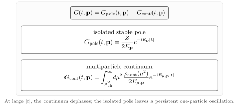
The large-time two-point function separates into a stable pole contribution and a multiparticle spectral integral. Here $E_{\mu,\mathbf p}=\sqrt{\mathbf p^2+\mu^2}$. The continuum dephases at large $|t|$, while the isolated pole leaves the persistent oscillation $Z e^{-iE_{\mathbf p}|t|}/(2E_{\mathbf p})$.

This is why the pole residue matters when Green functions are converted into scattering amplitudes: it tells us how strongly the chosen local field overlaps with the physical asymptotic particle. The residue is not by itself an observable—a field rescaling or a more general local field redefinition can change it—but LSZ uses precisely the compensating factors that make the final $S$-matrix independent of that choice.

The LSZ pole statement

Consider the connected momentum-space $N$-point function

$$\widetilde G_c^{(N)}(q_1,\ldots,q_N) =\int \prod_{j=1}^N d^4x_j\, \exp\left(i\sum_{j=1}^N q_j\cdot x_j\right) \langle0|T\phi(x_1)\cdots\phi(x_N)|0\rangle_c.$$

Translation invariance produces

$$(2\pi)^4\delta^{(4)}\left(\sum_{j=1}^N q_j\right).$$

For the physical process $1+2\to3+4$, choose

$$q_1=-p_1,\qquad q_2=-p_2,\qquad q_3=p_3,\qquad q_4=p_4.$$

Then $\sum_jq_j=0$ is exactly

$$p_1+p_2=p_3+p_4.$$

To see which assignment extracts the desired process, choose the state phases so that the overlap is $\sqrt Z>0$. At an incoming insertion the creation matrix element is $\langle p|\phi(x)|0\rangle=\sqrt Z e^{+ip\cdot x}$; at an outgoing insertion the annihilation matrix element is $\langle0|\phi(x)|p\rangle=\sqrt Z e^{-ip\cdot x}$. The corresponding LSZ weights are therefore $e^{-ip\cdot x}$ incoming and $e^{+ip\cdot x}$ outgoing. Comparing them with the declared forward transform gives the $q_j$ above.

Both $q_j^2=p_j^2$ and $\delta^{(4)}(-P)=\delta^{(4)}(P)$ hide a simultaneous reversal, so checking poles and total momentum conservation alone does not check the physical assignment. Tong, HTML edition 2021, § 3.7.2, Eq. (3.306) and the following reduction formula instead defines the forward transform with $e^{-i\sum q_j\cdot x_j}$; his incoming-positive/outgoing-negative arguments must be reversed when translated to the convention here.

Near the one-particle poles of all external legs, the connected four-point function has the universal form

$$\boxed{ \widetilde G_c^{(4)}(-p_1,-p_2,p_3,p_4) \simeq (2\pi)^4\delta^{(4)}(p_1+p_2-p_3-p_4) \left[\prod_{j=1}^4 {iZ^{1/2}\over p_j^2-M^2+i0}\right] i\mathcal M_{12\to34}. }$$

This equation is often the cleanest way to remember LSZ. A Green function has external poles because each field creates or destroys a one-particle state. The scattering amplitude is the finite coefficient that remains after those poles are removed.

The order of operations matters. One first multiplies by the inverse pole factors and only then takes the on-shell limit. Plugging $p_j^2=M^2$ into the unamputated Green function would hit the pole rather than extract its residue.

Equivalently, in the same convention,

$$\boxed{ i(2\pi)^4\delta^{(4)}(p_1+p_2-p_3-p_4)\mathcal M_{12\to34} = \left[ \prod_{j=1}^4 {p_j^2-M^2\over i\sqrt Z} \right] \widetilde G_c^{(4)}(-p_1,-p_2,p_3,p_4) \Big|_{\mathrm{on\ shell}}. }$$

This is the amputating operation: each factor $p_j^2-M^2$ removes the external pole, while each $Z^{-1/2}$ converts a field insertion into a normalized external particle.

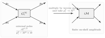
LSZ reduction removes the universal external pole factors from the connected Green function. The arrows carry physical momenta $p_j$; the left correlator is evaluated at $(-p_1,-p_2,p_3,p_4)$ in the stated Fourier convention. With the overall momentum delta suppressed, the result is the finite on-shell amplitude $i\mathcal M$.

A useful diagrammatic version is obtained by writing the connected four-point function near its poles as

$$\widetilde G_c^{(4)}(-p_1,-p_2,p_3,p_4) \simeq (2\pi)^4\delta^{(4)}(p_1+p_2-p_3-p_4) \left[\prod_{j=1}^4 {iZ\over p_j^2-M^2+i0}\right] i\Gamma_{\mathrm{amp}}^{(4)}.$$

Here $\Gamma_{\mathrm{amp}}^{(4)}$ is the full connected amputated four-point function, defined by removing the full external propagators but not yet normalizing external physical states. It includes contact and exchange contributions and should not be confused with only the 1PI four-point vertex of the effective action. Comparing with the LSZ pole statement gives

$$\boxed{ \mathcal M_{12\to34}=Z^2\Gamma_{\mathrm{amp}}^{(4)} }$$

for four external scalar particles. More generally, each external scalar contributes a factor $Z^{1/2}$ to the physical amplitude if the amputated vertex was defined using full propagators. The canonical LSZ derivation develops this distinction with the stable-state assumptions made explicit.

This is the bridge between the two languages used throughout perturbation theory: diagrams compute amputated Green functions, while experiments measure $|\mathcal M|^2$.

Invariant phase space

The final-state density of states must be Lorentz invariant. For one on-shell particle, the invariant measure is

$$d\Pi(p)={d^3\mathbf p\over (2\pi)^3 2E_{\mathbf p}}.$$

For $n$ final particles with total momentum $P$, define

$$\boxed{ d\Phi_n(P;p_1,\ldots,p_n) =(2\pi)^4\delta^{(4)}\left(P-\sum_{a=1}^n p_a\right) \prod_{a=1}^n {d^3\mathbf p_a\over (2\pi)^3 2E_a}. }$$

The delta function enforces total energy-momentum conservation; the product of measures counts Lorentz-invariant final states. This object is only the final-state measure. It does not include the initial flux factor, the squared amplitude, or possible symmetry factors for identical final particles.

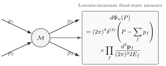
The amplitude $\mathcal M$ contains the dynamics. The invariant phase-space measure $d\Phi_n$ contains the universal kinematics and the energy-momentum conserving delta function.

For a decay of one particle $A$ with four-momentum $P$ into $n$ particles,

$$\boxed{ d\Gamma(A\to f) ={1\over S_f}{1\over 2E_A}|\mathcal M_{A\to f}|^2 d\Phi_n(P). }$$

In the rest frame of the decaying particle, $E_A=M_A$.

Here and below, $S_f$ removes overcounting of identical final particles. For example, if the phase-space integral labels two identical particles separately, then $S_f=2!$. For distinguishable final particles, $S_f=1$.

For two-particle scattering,

$$1+2\to f,$$

the differential cross section is

$$\boxed{ d\sigma ={1\over S_f} {|\mathcal M_{12\to f}|^2\over \mathcal F_{12}} \,d\Phi_f, \qquad \mathcal F_{12}=4\sqrt{(p_1\cdot p_2)^2-M_1^2M_2^2}. }$$

In a frame where the incoming beams are collinear, the invariant flux can also be written as

$$\mathcal F_{12}=4E_1E_2|\mathbf v_1-\mathbf v_2|, \qquad \mathbf v_a={\mathbf p_a\over E_a}.$$

The invariant form is the safest one outside simple beam or center-of-mass kinematics.

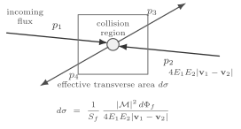
A cross section is a transition rate divided by incoming flux. The numerator is $|\mathcal M|^2$ times final-state phase space; the displayed velocity-difference denominator applies to the collinear incoming beams shown.

Two-body cross section

For a $2\to2$ process in the center-of-mass frame, let

$$s=(p_1+p_2)^2,$$

and write $|\mathbf p_i|$ for the magnitude of either incoming momentum and $|\mathbf p_f|$ for the magnitude of either outgoing momentum. The two-body phase space reduces to

$$d\Phi_2 ={1\over 16\pi^2}{|\mathbf p_f|\over \sqrt s}\,d\Omega.$$

The flux factor in the center-of-mass frame is

$$4E_1E_2|\mathbf v_1-\mathbf v_2| =4|\mathbf p_i|\sqrt s.$$

Therefore

$$\boxed{ {d\sigma\over d\Omega} ={1\over S_f}{1\over64\pi^2s} {|\mathbf p_f|\over |\mathbf p_i|} |\mathcal M|^2. }$$

For elastic scattering of equal-mass particles, $|\mathbf p_f|=|\mathbf p_i|$, so this simplifies to

$${d\sigma\over d\Omega} ={1\over S_f}{|\mathcal M|^2\over64\pi^2s}.$$

This compact formula is one reason the invariant amplitude is so useful. All the complicated dynamics is in $\mathcal M$; the rest is kinematics.

The φ⁴ check

Take a real scalar field with interaction

$$\mathcal L_{\mathrm{int}}=-{\lambda\over4!}\phi^4.$$

At tree level the four-point vertex gives

$$i\mathcal M=-i\lambda, \qquad \mathcal M=-\lambda.$$

The outgoing quanta of this real field are identical. If the direction of one labeled final momentum is integrated over the full sphere, the $1/2!$ symmetry factor gives

$${d\sigma\over d\Omega} ={\lambda^2\over128\pi^2s}{|\mathbf p_f|\over |\mathbf p_i|}.$$

For equal masses and elastic scattering,

$${d\sigma\over d\Omega}={\lambda^2\over128\pi^2s} \qquad\text{(full labeled solid angle)}.$$

Equivalently, omit the factor $1/2!$ and integrate over only one hemisphere, so that each unordered pair of final momenta is counted once. For a genuinely distinguishable contact-scattering process with the same constant amplitude, $S_f=1$ and the corresponding full-solid-angle formula has $64\pi^2s$ rather than $128\pi^2s$ in the denominator.

Summary

LSZ reduction is the statement that particles are poles of exact Green functions. Each external field insertion supplies a universal pole and a universal residue factor. Removing those external factors leaves the invariant amplitude $\mathcal M$.

The amplitude is not yet a probability. To obtain a physical observable, one squares $\mathcal M$, multiplies by invariant final-state phase space, and divides by the appropriate initial normalization: $2M$ for decay in the rest frame, or the relativistic flux factor for scattering.

Thus the conceptual chain is

$$\text{time-ordered Green function} \longrightarrow \text{amputated on-shell amplitude} \longrightarrow \text{rate or cross section}.$$

The next page changes viewpoint again: by Wick rotating to Euclidean time, the oscillatory path integral becomes a statistical-mechanics-like Gaussian measure.

Common pitfalls

• Forgetting the external $Z^{1/2}$ factors. Amputating propagators is not the same as normalizing external physical states. If the field is not already normalized so that $Z=1$, LSZ supplies a $Z^{-1/2}$ for each external field in the reduction formula, or equivalently $Z^{1/2}$ for each external particle in the amplitude built from an amputated vertex.
• Confusing Green functions with S-matrix elements. A time-ordered correlator is off shell and includes external propagators. The S-matrix amplitude is on shell and amputated.
• Dropping the flux factor. $|\mathcal M|^2d\Phi$ is a transition rate measure, not yet a cross section for a two-particle initial state.
• Double-counting identical final particles. The phase-space integral over labeled momenta counts identical configurations more than once unless a symmetry factor is included.
• Using nonrelativistic and relativistic normalizations in the same formula. The factors $2E_{\mathbf p}$ move between state normalizations, field overlaps, and phase-space measures.
• Setting external legs on shell too early. LSZ is a residue operation. Multiply by the inverse external propagators before taking the limit $p_j^2\to M^2$.
• Applying these formulas to unstable external particles. LSZ in this form assumes stable asymptotic one-particle states. Resonances are seen as poles of amplitudes, but they are not inserted as ordinary incoming or outgoing states.

Exercises

Exercise 1: two-body phase space

Derive the two-body phase-space formula

$$d\Phi_2 ={1\over16\pi^2}{|\mathbf p_f|\over\sqrt s}\,d\Omega$$

in the center-of-mass frame.

Solution

Start from

$$d\Phi_2 =(2\pi)^4\delta^{(4)}(P-p_3-p_4) {d^3\mathbf p_3\over(2\pi)^3 2E_3} {d^3\mathbf p_4\over(2\pi)^3 2E_4}.$$

In the center-of-mass frame,

$$P=(\sqrt s,\mathbf0).$$

The spatial delta function sets

$$\mathbf p_4=-\mathbf p_3.$$

Let $p=|\mathbf p_3|=|\mathbf p_4|$. Then

$$d^3\mathbf p_3=p^2dp\,d\Omega,$$

and

$$d\Phi_2 ={1\over(2\pi)^2}{p^2dp\,d\Omega\over4E_3E_4} \delta(\sqrt s-E_3(p)-E_4(p)).$$

Use

$${d\over dp}(E_3+E_4) =p\left({1\over E_3}+{1\over E_4}\right) ={p(E_3+E_4)\over E_3E_4} ={p\sqrt s\over E_3E_4}$$

on the support of the delta function. Hence

$$\int dp\,{p^2\over4E_3E_4}\delta(\sqrt s-E_3-E_4) ={p\over4\sqrt s}.$$

Therefore

$$d\Phi_2={1\over(2\pi)^2}{p\over4\sqrt s}d\Omega ={1\over16\pi^2}{|\mathbf p_f|\over\sqrt s}d\Omega.$$

Exercise 2: Residue factors from full amputation

Suppose the connected four-point function near its external poles is written as

$$\widetilde G_c^{(4)} \simeq (2\pi)^4\delta^{(4)}(p_1+p_2-p_3-p_4) \left[\prod_{j=1}^4 {iZ\over p_j^2-M^2+i0}\right] i\Gamma_{\mathrm{amp}}^{(4)}.$$

Using the LSZ pole statement on this page, determine $\mathcal M$ in terms of $\Gamma_{\mathrm{amp}}^{(4)}$.

Solution

The LSZ pole statement writes the same Green function as

$$\widetilde G_c^{(4)} \simeq (2\pi)^4\delta^{(4)}(p_1+p_2-p_3-p_4) \left[\prod_{j=1}^4 {iZ^{1/2}\over p_j^2-M^2+i0}\right] i\mathcal M.$$

Comparing the two expressions gives

$$\left[\prod_{j=1}^4 iZ\right]i\Gamma_{\mathrm{amp}}^{(4)} = \left[\prod_{j=1}^4 iZ^{1/2}\right]i\mathcal M.$$

The powers of $i$ are the same on both sides. The powers of $Z$ give

$$Z^4\Gamma_{\mathrm{amp}}^{(4)}=Z^2\mathcal M.$$

Thus

$$\boxed{\mathcal M=Z^2\Gamma_{\mathrm{amp}}^{(4)}.}$$

This is the four-external-leg version of the general rule: each external scalar contributes one factor $Z^{1/2}$ to the physical amplitude when the amputated vertex is defined by removing full propagators.

Exercise 3: two-body decay width

A scalar particle $A$ of mass $M$ decays into two identical scalar particles $B$ of mass $m$ through

$$\mathcal L_{\mathrm{int}}=-{g\over2}A B^2.$$

Assume $M>2m$, stable final particles $B$, and a weak coupling for which $\Gamma/M\ll1$. Compute the leading perturbative width of a prepared $A$ excitation. Here the cubic term is used as a perturbative interaction about a stable vacuum, with a stabilizing completion understood if needed; it is not a claim that the cubic potential alone is bounded below.

Solution

The vertex rule gives

$$i\mathcal M=-ig, \qquad |\mathcal M|^2=g^2.$$

For a one-particle decay in the rest frame,

$$d\Gamma={1\over2M}{1\over2!}|\mathcal M|^2d\Phi_2.$$

The factor $1/2!$ is required because the final particles are identical. From Exercise 1,

$$d\Phi_2={1\over16\pi^2}{|\mathbf p|\over M}d\Omega,$$

where

$$|\mathbf p|={M\over2}\sqrt{1-{4m^2\over M^2}}.$$

Integrating over $d\Omega$ gives

$$\int d\Phi_2={|\mathbf p|\over4\pi M}.$$

Therefore

$$\Gamma(A\to BB) ={1\over2M}{1\over2}g^2{|\mathbf p|\over4\pi M} ={g^2|\mathbf p|\over16\pi M^2}.$$

Substituting $|\mathbf p|$,

$$\boxed{ \Gamma(A\to BB) ={g^2\over32\pi M} \sqrt{1-{4m^2\over M^2}}. }$$

The result describes the approximately exponential regime of a narrow resonance, or equivalently its leading pole width. An unstable $A$ is not an exact infinite-time LSZ in-state. The decay-rate treatment states this time-window interpretation; at the earliest times a normalized state with finite energy variance instead has quadratic survival loss Crespi et al. 2019, arXiv v1, Eqs. (8)–(9), p. 3, PDF.

References

• Crespi, Andrea, Francesco V. Pepe, Paolo Facchi, Fabio Sciarrino, Paolo Mataloni, Hiromichi Nakazato, Saverio Pascazio, and Roberto Osellame. “Experimental Investigation of Quantum Decay at Short, Intermediate, and Long Times via Integrated Photonics.” Physical Review Letters 122 (2019), 130401. DOI. Open PDF, arXiv:1903.05378v1.
• Tong, David. Quantum Field Theory. University of Cambridge lecture notes, HTML edition, 2021. § 3.7.2, “From Green’s Functions to S-Matrices”.

Further reading

• Sidney Coleman, Lectures on Quantum Field Theory, edited by Bryan Gin-ge Chen et al., World Scientific, 2019, chapters 11–14.
• Michael E. Peskin and Daniel V. Schroeder, An Introduction to Quantum Field Theory, Addison-Wesley, 1995, chapters 4 and 7.
• Mark Srednicki, Quantum Field Theory, Cambridge University Press, 2007, sections 5, 10, and 11.
• Steven Weinberg, The Quantum Theory of Fields, Volume I: Foundations, Cambridge University Press, 1995, sections 3.4 and 10.3.