Superfluidity, Landau Criterion, and Accelerated Frames

A medium selects a rest frame, and a moving impurity can transfer energy and momentum to its excitations. The Landau criterion bounds when emission is energetically allowed; phase stiffness describes the fluid’s low-energy response. Rotating absorption and Rindler quantization provide two related applications of choosing a time-evolution generator, with different physical states and boundary conditions.

Our worked fluid is a uniform, weakly interacting neutral Bose gas in three spatial dimensions at zero temperature. We use one thermodynamic broken-symmetry representation. This choice is appropriate to that example; condensation and superfluid response are distinct diagnostics. The phase–density formulation supplies the canonical pair used below.

Energy in a moving frame

For a Galilean system in a sector of fixed total mass $\mathcal M$, a passive change to a frame moving with velocity $\mathbf v$ gives

$$E'=E-\mathbf v\cdot\mathbf P+\frac12\mathcal Mv^2.$$

The last term cancels between states in that sector. The generator relevant to excitation energies is therefore $H_{\mathbf v}=H-\mathbf v\cdot\mathbf P$. A fluid-rest-frame excitation with energy $\varepsilon(\mathbf p)>0$ has shifted energy

$$\varepsilon_{\mathbf v}(\mathbf p) =\varepsilon(\mathbf p)-\mathbf v\cdot\mathbf p.$$

A negative value means that this excitation lowers the shifted generator. It does not mean that relabeling coordinates creates a physical instability. Dissipation requires a subsystem, such as an impurity or boundary, that can exchange momentum, together with an allowed coupling and the appropriate conservation laws.

An active boost is a different operation. For a microscopic boson of mass $m$, giving a rest state velocity $\mathbf u$ acts as

$$\psi_{\mathbf u}(t,\mathbf x) =e^{im(\mathbf u\cdot\mathbf x-u^2t/2)} \psi(t,\mathbf x-\mathbf u t).$$

For a uniform rest condensate, the phase gradient becomes $\nabla\varphi+m\mathbf u$. The boosted state has laboratory momentum $\mathcal M\mathbf u$ and energy $E_0+\mathcal M u^2/2$. It is not another unconstrained laboratory ground state. Persistent flow is instead discussed at fixed momentum, imposed twist, or within a metastable winding sector.

The Landau threshold

Take an impurity of finite mass $M$, initially with momentum $\mathbf P=M\mathbf v$. If it emits one excitation of momentum $\mathbf p$, momentum and energy conservation require

$$\frac{\mathbf P^2}{2M} =\frac{|\mathbf P-\mathbf p|^2}{2M}+\varepsilon(\mathbf p), \qquad \mathbf v\cdot\mathbf p =\varepsilon(\mathbf p)+\frac{p^2}{2M}.$$

For fixed direction $\hat{\mathbf v}$, the corresponding energetic lower bound is

$$v_c(\hat{\mathbf v};M) =\inf_{\hat{\mathbf v}\cdot\mathbf p>0} \frac{\varepsilon(\mathbf p)+p^2/(2M)} {\hat{\mathbf v}\cdot\mathbf p}.$$

The recoil-free expression is the $M\to\infty$ limit. The direction in its denominator matters for anisotropic dispersion, as explained in Yu 2017, first preprint page, Eqs. (1)–(3), PDF. The finite-$M$ numerator follows from the conservation law just derived.

For an isotropic branch $\varepsilon=\varepsilon(p)$, alignment with the motion minimizes the ratio at fixed $p$. Thus

$$v_c(M)=\inf_{p>0}\left[\frac{\varepsilon(p)}p+\frac p{2M}\right], \qquad v_c(\infty)=\inf_{p>0}\frac{\varepsilon(p)}p.$$

If several excitation branches can couple, the infimum includes them all. These are energetic bounds for the specified emission channels, not decay rates. They do not decide vortex nucleation, boundary barriers or heating. Equality at an infimum also requires care: the minimizing nonzero momentum may not exist.

Two isotropic examples make that distinction explicit:

$$\varepsilon_B(p)=\sqrt{c_s^2p^2+\frac{p^4}{4m^2}}, \qquad \varepsilon_0(p)=\frac{p^2}{2m}.$$

The first is the Bogoliubov branch of the weak Bose model derived below; the second is an ideal noninteracting quadratic branch. Their ratios satisfy

$$\frac{\varepsilon_B(p)}p =\sqrt{c_s^2+\frac{p^2}{4m^2}}>c_s, \qquad \frac{\varepsilon_0(p)}p=\frac p{2m}>0 \quad(p>0).$$

As $p\downarrow0$, the bounds are $c_s$ and zero respectively, with neither attained at positive momentum. In the exactly linear phonon idealization $\varepsilon=c_sp$, by contrast, every positive momentum attains the recoil-free ratio $c_s$. Finite recoil adds $p/(2M)$, making its threshold unattained as well. For that model the most favorable emission is collinear:

$$v=c_s+\frac p{2M},$$

so any nonzero emitted momentum requires $v>c_s$.

The figure separates the dispersion from its ratio to momentum. Both panels use $q=p/(2mc_s)$; the same positive $c_s$ is merely a comparison scale for the ideal branch.

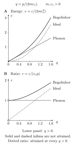
The Landau bound uses slopes from the origin, shown explicitly as $\varepsilon/(c_sp)$ below. The physical ratio $\varepsilon/p$ has infimum $c_s$ for the Bogoliubov branch and zero for the ideal quadratic branch; neither is attained at nonzero momentum. The dotted linear phonon model has $\varepsilon/p=c_s$ at every positive momentum, so its normalized ratio is 1. The same $m,c_s$ define the comparison units; the ideal branch is not assigned a sound speed. These exact isotropic branch plots omit impurity recoil and do not predict a decay rate or vortex threshold.

Editable TikZ source. Original diagram for QFT.org, created with OpenAI Codex and licensed under CC BY 4.0.

The moving-fluid convention in Altland and Simons 2023, §5.2.4, p. 257 shifts energies by $+\mathbf V\cdot\mathbf p$. Relative to our impurity motion, $\mathbf V=-\mathbf v$, so the emission sign agrees.

Density and phase form one canonical pair

For the weak repulsive Bose model, write $\psi=\rho e^{i\varphi}$ and $n=\rho^2$. The static grand-potential functional is

$$F[\psi]=\int d^3x\left[ \frac{|\nabla\psi|^2}{2m}-\mu|\psi|^2+\frac g2|\psi|^4 \right], \qquad g>0,\quad\mu>0.$$

Its uniform minimum has

$$n_0=\rho_0^2=\frac\mu g, \qquad U(\rho)=-\mu\rho^2+\frac g2\rho^4, \qquad U''(\rho_0)=4\mu>0.$$

This is a positive static radial curvature. To identify dynamical modes we must also retain the time derivative. Dropping a total derivative from the microscopic Bose action gives

$$\mathcal L=-n\dot\varphi -\frac{n}{2m}(\nabla\varphi)^2 -\frac{(\nabla n)^2}{8mn} +\mu n-\frac g2n^2.$$

The term $-n\dot\varphi$ makes density and phase conjugate variables. Expand $n=n_0+\delta n$; the linear density term cancels because $\mu=gn_0$. Apart from the background phase derivative, the quadratic Lagrangian is

$$\mathcal L_2= -\delta n\,\dot\varphi-\frac g2(\delta n)^2 -\frac{n_0}{2m}(\nabla\varphi)^2 -\frac{(\nabla\delta n)^2}{8mn_0}.$$

The conjugate-pair and long-wavelength derivation is developed in Altland and Simons 2023, §5.2.4, pp. 254–257, especially Eqs. (5.13)–(5.15). Their density variable is our $n$, and the quadratic density cost here means $(\delta n)^2$ after the chemical-potential tadpole is canceled. Their Euclidean Berry term $i\delta n\,\partial_\tau\varphi$ continues to the real-time sign above.

At momenta small compared with the inverse healing scale, the last gradient term is subleading. Completing the square,

$$-\delta n\,\dot\varphi-\frac g2(\delta n)^2 =-\frac g2\left(\delta n+\frac{\dot\varphi}{g}\right)^2 +\frac{(\dot\varphi)^2}{2g},$$

gives the phase action

$$\begin{gathered} S_{\rm ph}=\frac12\int dt\,d^3x \left[\chi(\partial_t\varphi)^2-n_s(\nabla\varphi)^2\right],\\ \chi=\frac{\partial n}{\partial\mu}=\frac1g, \qquad n_s=\frac{n_0}{m}. \end{gathered}$$

Here $n_s$ denotes stiffness, not number density. The sound speed is

$$c_s^2=\frac{n_s}{\chi}=\frac{gn_0}{m}.$$

Retaining the density-gradient term gives two first-order equations,

$$\dot\varphi=-\left(g-\frac{\nabla^2}{4mn_0}\right)\delta n, \qquad \dot{\delta n}=-\frac{n_0}{m}\nabla^2\varphi.$$

Combining them yields

$$\omega^2= \left(g+\frac{k^2}{4mn_0}\right)\frac{n_0k^2}{m} =c_s^2k^2+\frac{k^4}{4m^2}.$$

There is one positive-frequency Bogoliubov branch and its negative-frequency partner. Positive radial curvature did not supply a second, independently gapped amplitude mode. The full displayed dispersion belongs to the quadratic weak-Bose approximation; its high-momentum validity is limited by the microscopic interaction model.

The selected phase also needs its thermodynamic scope. At finite volume a number eigenstate has $\langle\psi\rangle=0$. A definite condensate phase is obtained by taking the thermodynamic limit before removing a symmetry-breaking source. Superfluid stiffness and condensation need not coincide in other dimensions or regimes; see Altland and Simons 2023, §5.2, p. 242, and §5.2.4, p. 254.

Source response and fixed winding

Couple the conserved particle-number symmetry to a background one-form $a=a_0dt+a_i dx^i$, with charge $Q$. Its transformation is

$$\varphi\mapsto\varphi+Q\lambda,\qquad a_\mu\mapsto a_\mu+\partial_\mu\lambda,\qquad D_\mu\varphi=\partial_\mu\varphi-Qa_\mu.$$

The spatial $a_i$ are covector components in this source convention. They are not silently identified with a raised Lorentzian electromagnetic vector. Cartesian spatial current labels below use $\delta_{ij}$; they do not mean Lorentzian index lowering.

At long wavelengths, expand about the chosen rest density. The density–phase action contains

$$\mathcal L= -n_0D_0\varphi-\delta nD_0\varphi -\frac g2(\delta n)^2 -\frac{n_s}{2}(D_i\varphi)^2+\cdots.$$

In particular, $Qn_0a_0$ supplies the equilibrium density response. Eliminating $\delta n$ gives

$$S[\varphi,a]=\int dt\,d^3x \left[-n_0D_0\varphi+ \frac{\chi}{2}(D_0\varphi)^2 -\frac{n_s}{2}(D_i\varphi)^2\right].$$

The background derivative $-n_0\dot\varphi$ does not alter local equations in a fixed smooth sector; global compact-phase sectors require separate treatment. It may be omitted in a fluctuation action only if the equilibrium current is stated separately. Functional differentiation gives

$$j^0=\frac{\delta S}{\delta a_0} =Qn_0-Q\chi D_0\varphi, \qquad j^i=\frac{\delta S}{\delta a_i} =Qn_sD_i\varphi.$$

At zero source the phase equation has the sound pole

$$D(\omega,\mathbf k)= \chi(\omega+i0)^2-n_sk^2.$$

Varying the phase gives

$$\chi\partial_tD_0\varphi-n_s\partial_iD_i\varphi=0.$$

For inverse Fourier phase $e^{-i\omega t+i\mathbf k\cdot\mathbf x}$, set $z=\omega+i0$. The retarded solution is

$$\varphi(z,\mathbf k)= \frac{iQ(\chi z a_0+n_s\mathbf k\cdot\mathbf a)} {\chi z^2-n_sk^2}.$$

Substituting into $j_i=Qn_s(ik_i\varphi-Qa_i)$ gives the retarded spatial current response $R_{ij}=\delta j_i/\delta a_j$:

$$R_{ij}(\omega,\mathbf k) =-Q^2n_s\delta_{ij} -\frac{Q^2n_s^2k_i k_j}{\chi z^2-n_sk^2}.$$

The first term is a source contact term and the second is phase exchange. Their combination, not the pole alone, gives the static limit.

To see that limit directly, minimize

$$F[\varphi,a]=\frac{n_s}{2} \int d^3x\,(\nabla\varphi-Q\mathbf a)^2.$$

Work at nonzero spatial momentum, with vanishing boundary terms and single-valued smooth phase variations in the zero-winding sector of the rest state. Decompose

$$a_i=a_i^{\rm T}+\partial_i\lambda, \qquad \partial_i a_i^{\rm T}=0.$$

For the exact longitudinal component removable within that sector, $\varphi=Q\lambda$ gives

$$F_{\min}[a]=\frac{n_sQ^2}{2}\int d^3x\,(a_i^{\rm T})^2.$$

Define the positive static Hessian $K$, and the induced current about the zero-source rest state, by

$$\begin{aligned} K_{ij}(\mathbf k) &=\frac{\delta^2F_{\min}} {\delta a_i(-\mathbf k)\delta a_j(\mathbf k)} =n_sQ^2\left(\delta_{ij}-\frac{k_i k_j}{k^2}\right),\\ j_i(\mathbf k)&=-\frac{\delta F_{\min}}{\delta a_i(-\mathbf k)} =-K_{ij}(\mathbf k)a_j(\mathbf k), \qquad \mathbf k\ne0. \end{aligned}$$

Thus $R_{ij}(0,\mathbf k)=-K_{ij}(\mathbf k)$. The local contact and the phase-exchange term cancel the longitudinal response. The $k_i k_j/k^2$ structure is nonanalytic at zero momentum, so the zero mode cannot be inferred by substituting $k=0$.

A ring makes the global exception concrete. For circumference $L$, uniform cross-sectional area $\mathcal A_\perp$, constant tangential source $a$, and fixed winding $w\in\mathbb Z$,

$$F_w(a)=\frac{n_s\mathcal A_\perp L}{2} \left(\frac{2\pi w}{L}-Qa\right)^2.$$

The candidate phase $Qax$ is not generally single-valued modulo $2\pi$ around the ring. A nontrivial holonomy therefore cannot be discarded as an ordinary longitudinal fluctuation. Changing $w$ involves physics outside this smooth-sector minimization.

The background-source calculation describes a neutral fluid’s sound and stiffness. With an appropriately normalized dynamical Maxwell field, the charged phase instead participates in the Anderson–Higgs mechanism and transverse stiffness contributes to Meissner screening. This requires the electromagnetic dynamics; a nondynamical probe alone does not remove the neutral phonon.

Rotating absorption

A rotating system uses the generator $H_\Omega=H-\Omega L_z$. Write $\ell$ for the angular-momentum quantum number, so it is not confused with the particle mass. A bosonic mode with laboratory frequency $\omega>0$ has corotating frequency

$$\omega_{\rm co}=\omega-\ell\Omega.$$

Consider an axisymmetric body at constant angular velocity, internally equilibrated, with a dissipative channel coupled to this mode. Absorbed energy and angular momentum are in the ratio $\omega:\ell$. Positivity of dissipation in the rotating frame constrains the signed absorption fraction $\mathcal A_\ell$:

$$(\omega-\ell\Omega)\mathcal A_\ell\ge0.$$

When $0<\omega<\ell\Omega$ and the channel has nonzero dissipative coupling, $\mathcal A_\ell<0$: outgoing power exceeds incident power by extracting rotational energy. A decoupled channel with $\mathcal A_\ell=0$ is not amplified. This is the rotating-body argument in Bekenstein and Schiffer 1998, §IV, preprint pp. 10–12, Eqs. (21)–(26), PDF, using $\ell$ for their $m$.

The shifted energy resembles $\varepsilon-\mathbf v\cdot\mathbf p$, but the absorption and boundary conditions carry the physical content. The sign by itself is not a theorem of fermionic amplification or a substitute for the flux analysis of a particular horizon problem.

Accelerated coordinates and the vacuum state

In the right wedge $x>|t|$ of $1+1$-dimensional Minkowski space, introduce

$$t=\rho\sinh\eta,\qquad x=\rho\cosh\eta,\qquad \rho>0.$$

Differentiating and canceling the cross terms gives

$$ds^2=dt^2-dx^2=\rho^2d\eta^2-d\rho^2.$$

At fixed $\rho$ the worldline satisfies $x^2-t^2=\rho^2$, with proper time and proper acceleration

$$d\tau_{\rm prop}=\rho\,d\eta, \qquad a_{\rm prop}=\frac1\rho.$$

Rindler time $\eta$ is dimensionless boost time. A factor $e^{-i\omega\eta}$ therefore has dimensionless boost frequency $\omega$, while the observer measures proper frequency $\omega/\rho$.

With $\eta=-i\theta$, the Euclidean metric is

$$ds_E^2=d\rho^2+\rho^2d\theta^2.$$

Regularity at the origin of the Euclidean plane requires $\theta\sim\theta+2\pi$. For the analytic Minkowski vacuum, this angular continuation yields the wedge KMS period $2\pi$ in boost time. The observer at fixed $\rho$ has

$$\beta_{\rm prop}=2\pi\rho, \qquad T_{\rm U}=\frac1{2\pi\rho} =\frac{a_{\rm prop}}{2\pi}.$$

The state assumption is essential. An arbitrary state in the wedge, including the Rindler vacuum, does not become thermal merely through a coordinate change. The analytic, Poincaré-vacuum/Wightman setting and Euclidean argument are discussed in Crispino, Higuchi and Matsas 2007, §II.I, preprint pp. 16–18, PDF. This statement concerns wedge correlation functions and boost evolution; it does not require a literal trace-class density matrix for an unregulated continuum wedge.

Massive Rindler modes

For a real scalar of mass $m>0$, the action and equation of motion are

$$S=\frac12\int dt\,dx \left[(\partial_t\phi)^2-(\partial_x\phi)^2-m^2\phi^2\right],$$ $$\left[ \frac1{\rho^2}\partial_\eta^2 -\frac1\rho\partial_\rho(\rho\partial_\rho)+m^2 \right]\phi=0.$$

Introduce a reference length $\rho_0>0$ and $z=\log(\rho/\rho_0)$. Then

$$\begin{gathered} ds^2=\rho_0^2e^{2z}(d\eta^2-dz^2),\\ S=\frac12\int d\eta\,dz \left[(\partial_\eta\phi)^2-(\partial_z\phi)^2 -(m\rho_0)^2e^{2z}\phi^2\right]. \end{gathered}$$

The conjugate momentum is $\pi=\partial_\eta\phi$, so the boost Hamiltonian is

$$H_R=\frac12\int dz \left[\pi^2+(\partial_z\phi)^2 +(m\rho_0)^2e^{2z}\phi^2\right].$$

For real positive boost frequency, set $\phi=e^{-i\omega\eta}f_\omega(z)$ with $\omega>0$. The mode equation becomes

$$\left[\partial_z^2+\omega^2-(m\rho_0)^2e^{2z}\right]f_\omega(z)=0.$$

The mass produces an exponential wall. Choosing a radial mode real and decaying as $\rho\to\infty$ gives

$$f_\omega(z)=K_{i\omega}(m\rho_0e^z) =K_{i\omega}(m\rho).$$

Near the horizon the wall vanishes. The small-argument Bessel expansion explicitly gives

$$\begin{aligned} K_{i\omega}(m\rho_0e^z) &\sim\frac12\Gamma(i\omega) \left(\frac{m\rho_0}{2}\right)^{-i\omega}e^{-i\omega z} \\ &\quad+\frac12\Gamma(-i\omega) \left(\frac{m\rho_0}{2}\right)^{i\omega}e^{i\omega z}. \end{aligned}$$

The coefficients are complex conjugates for the stated real parameters. The overall Klein–Gordon normalization is not fixed by choosing this radial profile. For $m=0$ there is no exponential wall, and this decaying massive boundary condition must be replaced.

These modes are the zero-transverse-momentum specialization of Crispino, Higuchi and Matsas 2007, §§II.D–E, preprint pp. 10–11, Eqs. (2.84)–(2.106), PDF. If their acceleration scale and coordinates are $a_s,\tau,\xi$, the translation is $\rho=e^{a_s\xi}/a_s$, $\eta=a_s\tau$, and $\omega=\omega_s/a_s$. Their four-dimensional transverse normalization is not being reused here.

Positive boost frequency and positive Minkowski frequency specify different mode decompositions. The Minkowski vacuum requires an analytic combination across the wedges. In a canonically normalized Rindler basis, its occupation factor is $(e^{2\pi\omega}-1)^{-1}$; the Rindler vacuum uses zero-temperature boost occupations. Changing the time generator is therefore only part of the question: the state and its analyticity determine the occupation and KMS properties.

Common pitfalls

An energetic bound is not a rate. The Landau and rotating-frame inequalities need a physical exchange or dissipative channel. A passive coordinate change supplies neither.

Static curvature does not count dynamical modes. In the weak nonrelativistic Bose fluid, density and phase are a conjugate pair and generate the Bogoliubov branch.

A transverse response requires its contact term and global scope. The Hessian is positive, while the induced static current is its negative action on the source. A fixed-winding holonomy is not removed by an arbitrary phase gradient.

Unruh thermality is a state statement. The temperature above applies to the Minkowski vacuum and proper-time normalization, not to every accelerated state.

The remaining limitation of the smooth fluid description is topological. The phase obeys $\varphi\sim\varphi+2\pi$; winding changes and vortices require more than small real-valued phase fluctuations. The next lesson starts from this compactness. Its Euclidean probe absorbs the charge into the source, whereas the single-boson normalization here keeps $Q$ explicit.

Exercises

A dispersion whose bound is not attained

In an isotropic continuum model with no recoil or momentum cutoff, let a quasiparticle have dispersion

$$\varepsilon(p)=\sqrt{\Delta^2+c^2p^2}.$$

Assume $\Delta>0$ and $c>0$. Compute the Landau critical velocity

$$v_c=\inf_{p>0}{\varepsilon(p)\over p}.$$

Interpret the result.

Solution

We have

$${\varepsilon(p)\over p}=\sqrt{{\Delta^2\over p^2}+c^2}.$$

For $\Delta>0$, this decreases monotonically as $p$ increases and approaches $c$ from above:

$$\lim_{p\to\infty}{\varepsilon(p)\over p}=c.$$

Thus the infimum is

$$v_c=c.$$

This result should be interpreted with care. The relativistic-looking dispersion has no finite-momentum minimum of $\varepsilon/p$; only its infimum is approached asymptotically. In a real condensed-matter system the high-momentum dispersion will eventually deviate from this form, and the actual minimum may occur elsewhere. The exercise shows both why the full dispersion matters and why the criterion is best written with an infimum.

Finite recoil in phonon emission

A body of finite mass $M>0$ moves with velocity $\mathbf v$ through an unbounded homogeneous fluid. Assume an isotropic excitation branch and continuously variable momentum, with no infrared cutoff. Keeping the recoil term, show that emission of a quasiparticle with momentum $\mathbf k$ requires

$$\mathbf v\cdot\mathbf k=\varepsilon(\mathbf k)+{\mathbf k^2\over2M}.$$

For the ideal phonon branch $\varepsilon(k)=c_s k$, with $c_s>0$, find the infimum of speeds that permit emission at finite $M$, and state whether it is attained at nonzero $k$.

Solution

Energy conservation gives

$${\mathbf P^2\over2M}={|\mathbf P-\mathbf k|^2\over2M}+\varepsilon(\mathbf k).$$

Expanding the square,

$$|\mathbf P-\mathbf k|^2=\mathbf P^2-2\mathbf P\cdot\mathbf k+\mathbf k^2.$$

Therefore

$$0={-2\mathbf P\cdot\mathbf k+\mathbf k^2\over2M}+\varepsilon(\mathbf k),$$

or

$${\mathbf P\over M}\cdot\mathbf k=\varepsilon(\mathbf k)+{\mathbf k^2\over2M}.$$

Since $\mathbf v=\mathbf P/M$,

$$\mathbf v\cdot\mathbf k=\varepsilon(\mathbf k)+{\mathbf k^2\over2M}.$$

For phonons,

$$v k\cos\theta=c_s k+{k^2\over2M}.$$

The most favorable angle is $\cos\theta=1$, so

$$v=c_s+{k\over2M}.$$

For any finite $k$ this is larger than $c_s$, but by taking $k\to0$ one approaches

$$v_c=c_s.$$

Thus recoil does not change the infimum of the threshold in the ideal phonon theory, although no finite-$k$ emission occurs exactly at $v=c_s$ and recoil changes the kinematics at every fixed nonzero $k$.

Euclidean regularity of Rindler space

In the right Minkowski wedge with $\rho>0$, derive the Rindler metric from

$$t=\rho\sinh\eta, \qquad x=\rho\cosh\eta.$$

Then analytically continue $\eta=-i\theta$ and require a smooth Euclidean plane including $\rho=0$. Show that regularity requires $\theta$ to have period $2\pi$.

Solution

Differentiate:

$$dt=\sinh\eta\,d\rho+\rho\cosh\eta\,d\eta,$$ $$dx=\cosh\eta\,d\rho+\rho\sinh\eta\,d\eta.$$

Then

$$dt^2-dx^2 =(\sinh^2\eta-\cosh^2\eta)d\rho^2 +\rho^2(\cosh^2\eta-\sinh^2\eta)d\eta^2,$$

while the cross terms cancel. Since

$$\cosh^2\eta-\sinh^2\eta=1,$$

we get

$$ds^2=\rho^2d\eta^2-d\rho^2.$$

Set $\eta=-i\theta$. The Euclidean metric is

$$ds_E^2=d\rho^2+\rho^2d\theta^2.$$

This is the flat plane in polar coordinates. At $\rho=0$, the coordinate $\theta$ is an angle. The plane is smooth only if

$$\theta\sim\theta+2\pi.$$

A different period would produce a conical singularity.

Rindler mode equation

Starting from the massive Klein–Gordon equation in Rindler coordinates,

$$\left[{1\over\rho^2}\partial_\eta^2-{1\over\rho}\partial_\rho(\rho\partial_\rho)+m^2\right]\phi=0,$$

take $m>0$, $\rho_0>0$ and real boost frequency $\omega>0$, and set $\rho=\rho_0e^z$ and $\phi=e^{-i\omega\eta}f_\omega(z)$. Show that

$$\left(\partial_z^2+\omega^2-(m\rho_0)^2e^{2z}\right)f_\omega(z)=0.$$

Solution

Since $\rho=\rho_0e^z$,

$$\partial_\rho={1\over\rho}\partial_z.$$

Therefore

$$\rho\partial_\rho=\partial_z,$$

and

$${1\over\rho}\partial_\rho(\rho\partial_\rho) ={1\over\rho}\partial_\rho\partial_z ={1\over\rho^2}\partial_z^2.$$

Substituting into the wave equation gives

$$\left[{1\over\rho^2}\partial_\eta^2-{1\over\rho^2}\partial_z^2+m^2\right]\phi=0.$$

Multiplying by $\rho^2=\rho_0^2e^{2z}$,

$$\left[\partial_\eta^2-\partial_z^2+(m\rho_0)^2e^{2z}\right]\phi=0.$$

With $\phi=e^{-i\omega\eta}f_\omega(z)$,

$$\left[-\omega^2-\partial_z^2+(m\rho_0)^2e^{2z}\right]f_\omega(z)=0.$$

Multiplying by $-1$ gives

$$\left(\partial_z^2+\omega^2-(m\rho_0)^2e^{2z}\right)f_\omega(z)=0.$$

Static transverse response

Use the background spatial one-form components $a_i$ of the main text. Work in the smooth zero-winding sector, with boundary conditions making the integrations by parts below valid. Assume the longitudinal source is globally exact, $a_i^{\rm L}=\partial_i\lambda$, with $Q\lambda$ an allowed single-valued phase variation. Consider the phase-only free energy

$$F[\varphi,a]={n_s\over2}\int d^d x\,(\nabla\varphi-Q\mathbf a)^2.$$

Decompose $\mathbf a=\mathbf a^{\rm T}+\nabla\lambda$ with $\nabla\cdot\mathbf a^{\rm T}=0$. Minimize over $\varphi$ and show that only the transverse field costs energy.

Solution

Substitute the decomposition:

$$\nabla\varphi-Q\mathbf a =\nabla\varphi-Q\nabla\lambda-Q\mathbf a^{\rm T} =\nabla(\varphi-Q\lambda)-Q\mathbf a^{\rm T}.$$

The transverse field is orthogonal to gradients under integration by parts:

$$\int d^d x\,\mathbf a^{\rm T}\cdot\nabla f =-\int d^d x\,f\,\nabla\cdot\mathbf a^{\rm T}=0,$$

assuming boundary terms vanish. Therefore

$$F={n_s\over2}\int d^d x\, \left[(\nabla(\varphi-Q\lambda))^2+Q^2(\mathbf a^{\rm T})^2\right].$$

The minimum over $\varphi$ is obtained by choosing

$$\varphi=Q\lambda+\text{constant},$$

so

$$F_{\rm min}[a]={n_s Q^2\over2}\int d^d x\,(\mathbf a^{\rm T})^2.$$

Thus the phase screens the longitudinal part of $\mathbf a$, while the transverse part measures the stiffness. This is the static origin of the superfluid or superconducting current response.

References

• Altland, A., and Simons, B. Condensed Matter Field Theory. 3rd ed. Cambridge University Press, 2023. DOI.
• Bekenstein, J. D., and Schiffer, M. “The Many Faces of Superradiance.” Physical Review D 58 (1998): 064014. DOI. Open PDF: preprint v1.
• Crispino, L. C. B., Higuchi, A., and Matsas, G. E. A. “The Unruh Effect and Its Applications.” Reviews of Modern Physics 80 (2008): 787–838. arXiv record. Open PDF: preprint v1, 2007.
• Yu, Z.-Q. “Landau Criterion for an Anisotropic Bose–Einstein Condensate.” Physical Review A 95 (2017): 033618. DOI. Open PDF: preprint v1.