Interacting Bose Fields and Bogoliubov Sound

Free bosons are deceptively simple. A macroscopic number of them can sit in the same one-particle state, and the energy of a particle with small momentum is only $\mathbf p^2/(2m)$. This produces an enormous supply of very low-energy excitations. A weak repulsive interaction changes the situation qualitatively: the low-energy excitation is no longer a single particle moving through an inert background, but a collective density wave. Its energy is linear at small momentum,

$$\omega_{\mathbf k}\simeq c|\mathbf k|,$$

so the interacting Bose gas has sound.

This page develops that result for a homogeneous three-dimensional Bose gas at zero temperature, on a stable weakly repulsive gas branch. The field obeys the equal-time commutator introduced earlier. In a coherent or selected-phase description, small fluctuations about the condensate mix particles with holes and produce the Bogoliubov spectrum. We then calculate the noncondensate population to test whether the approximation is self-consistent.

Interacting Bose Hamiltonian

Repulsive contact gas at fixed chemical potential

We continue to use the nonrelativistic equal-time normalization

$$[\psi(\mathbf x),\psi^\dagger(\mathbf y)]=\delta^{(3)}(\mathbf x-\mathbf y).$$

The particle density operator is $\hat n(\mathbf x)=\psi^\dagger(\mathbf x)\psi(\mathbf x)$. For the contact interaction we write $g>0$ for repulsion. To study a static condensate it is convenient to use the grand-canonical Hamiltonian $K=H-\mu N$.

The most natural nonrelativistic interaction is a pair potential. For identical bosons described by the field $\psi(\mathbf x)$, the Hamiltonian is

$$H=\int d^3x\,\frac{1}{2m}\nabla\psi^\dagger\cdot\nabla\psi +\frac12\int d^3x\,d^3y\,V(\mathbf x-\mathbf y) \psi^\dagger(\mathbf x)\psi^\dagger(\mathbf y) \psi(\mathbf y)\psi(\mathbf x).$$

The factor $1/2$ avoids double-counting pairs. The ordering shown here is normal ordered: annihilation operators stand to the right of creation operators. For smooth $V$, this Hamiltonian is the second-quantized version of the many-body Hamiltonian

$$H_N=\sum_{i=1}^N\left(-\frac{\nabla_i^2}{2m}\right) +\sum_{1\leq i<j\leq N}V(\mathbf x_i-\mathbf x_j).$$

The Heisenberg equation

$$i\partial_t\psi(\mathbf x,t)=[\psi(\mathbf x,t),H]$$

gives

$$i\partial_t\psi(\mathbf x,t) =-\frac{\nabla^2}{2m}\psi(\mathbf x,t) +\int d^3y\,V(\mathbf x-\mathbf y) \psi^\dagger(\mathbf y,t)\psi(\mathbf y,t)\psi(\mathbf x,t).$$

This equation is still exact as an operator equation. It already has the form of a Schrödinger equation in a self-consistent potential: the particle annihilated at $\mathbf x$ feels the density of all other particles.

A particularly important idealization is a short-range repulsion,

$$V(\mathbf x-\mathbf y)=g\delta^{(3)}(\mathbf x-\mathbf y), \qquad g>0.$$

Then the contact Hamiltonian should be read as the normal-ordered operator

$$H=\int d^3x\left[\frac{1}{2m}\nabla\psi^\dagger\cdot\nabla\psi +\frac g2\psi^\dagger\psi^\dagger\psi\psi\right] =\int d^3x\left[\frac{1}{2m}\nabla\psi^\dagger\cdot\nabla\psi +\frac g2:(\psi^\dagger\psi)^2:\right].$$

With this understood, the equation of motion becomes

$$i\partial_t\psi =-\frac{\nabla^2}{2m}\psi+g\psi^\dagger\psi\,\psi.$$

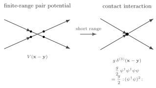
The contact term $g\psi^\dagger\psi^\dagger\psi\psi/2= g:(\psi^\dagger\psi)^2:/2$ represents a local two-body repulsion. In perturbation theory it becomes a four-leg vertex; in mean-field theory it becomes an energy cost proportional to the square of the density.

The contact interaction is a low-energy effective description. In three spatial dimensions its matched coupling is $g=4\pi a/m$, where $a>0$ is the two-body scattering length and $m>0$. This is not an identification of an arbitrary bare cutoff coupling with $4\pi a/m$: the regulated interaction must reproduce the physical scattering length. The regularized pseudopotential and its matching are given in Castin 2001, arXiv v1, § 3.2.1, p. 28, Eqs. (73)–(74), PDF. We assume a stable dilute gas branch; positive scattering length alone does not establish microscopic ground-state stability. The matched weak-gas action explains the same coupling convention.

The large-occupation classical limit

Large occupation can help justify a classical approximation, but the state matters. For a single oscillator mode,

$$[a,a^\dagger]=1, \qquad N=a^\dagger a.$$

For a state with finite, nonzero mean occupation $\langle N\rangle$, the ratio of expectations is

$$\frac{\langle[a,a^\dagger]\rangle}{\langle a^\dagger a\rangle} =\frac{1}{\langle N\rangle}.$$

This compares two numbers; it does not divide by the number operator, which has a zero eigenvalue. The ratio becomes small at large mean occupation, but it does not establish coherence. In a coherent state $a|\alpha\rangle=\alpha|\alpha\rangle$, one has $\langle N\rangle=|\alpha|^2$ and relative number fluctuation $\Delta N/\langle N\rangle=1/\sqrt{\langle N\rangle}$. A number eigenstate instead has $\langle a\rangle=0$, however large its occupation.

For a Bose field, an extensive occupation of one orbital likewise need not give a nonzero $\langle\psi\rangle$: at fixed total particle number, $\psi$ changes that number and its expectation vanishes. A coherent or selected thermodynamic phase permits the classical order parameter below. A number-conserving treatment describes condensation without requiring that expectation value; see Castin 2001, arXiv v1, § 7, pp. 86–88, PDF and the distinction between condensation and a selected phase. In the selected-phase description, write

$$\Psi(\mathbf x,t)=\langle\psi(\mathbf x,t)\rangle.$$

Replacing $\psi$ by $\Psi$ in the contact-interaction Hamiltonian gives the Gross–Pitaevskii energy functional

$$E[\Psi]=\int d^3x\left[ \frac{1}{2m}|\nabla\Psi|^2+\frac g2|\Psi|^4 \right].$$

In this classical functional, $N$ denotes the conserved saddle-order condensate population. Its normalization is

$$N=\int d^3x\,|\Psi|^2.$$

To fix the average density it is convenient to minimize

$$K[\Psi]=E[\Psi]-\mu N =\int d^3x\left[ \frac{1}{2m}|\nabla\Psi|^2-\mu|\Psi|^2+\frac g2|\Psi|^4 \right].$$

For a uniform field $\Psi=\sqrt n\,e^{i\theta}$, the grand-canonical energy density is

$$\mathcal E_\mu(n)=-\mu n+\frac g2 n^2 =\frac g2\left(n-\frac{\mu}{g}\right)^2-\frac{\mu^2}{2g}.$$

For $g>0$ and $\mu>0$ the mean-field minimum occurs at the leading Gross–Pitaevskii density

$$n_0=\frac{\mu}{g}.$$

The sign restriction is physical. If the same contact model is continued to $g<0$, the quartic energy is unbounded below at fixed chemical potential, and the uniform dilute-gas saddle is not stable without additional physics. In the linearized spectrum below, the same instability appears as $\omega_k^2<0$ at sufficiently small $k$. We therefore keep $g>0$ throughout the sound-mode derivation.

The phase $\theta$ is arbitrary. Choosing one value of $\theta$ is the mean-field signal of spontaneous breaking of the global $U(1)$ symmetry

$$\psi\mapsto e^{-i\alpha}\psi.$$

The broken symmetry does not mean that particle number has disappeared from the exact theory. The exact Hamiltonian still commutes with

$$N=\int d^3x\,\psi^\dagger\psi.$$

A selected phase is obtained by taking the thermodynamic limit before removing an infinitesimal symmetry-breaking source. It is not the field expectation in a finite-volume number eigenstate. Small changes of the selected phase become the low-energy collective mode.

The classical equation of motion in the grand-canonical frame is

$$i\partial_t\Psi =-\frac{\nabla^2}{2m}\Psi-\mu\Psi+g|\Psi|^2\Psi.$$

The uniform condensate

$$\Psi_0=\sqrt{n_0}$$

is time independent in this leading Gross–Pitaevskii equation because $\mu=gn_0$. Without subtracting $\mu N$, the same mean-field condensate would rotate in phase as $\Psi(t)=\sqrt{n_0}e^{-i\mu t}$.

Linearization around the condensate

Choose the condensate phase so that $\Psi_0=\sqrt{n_0}$ is real, and write the operator field as

$$\psi(\mathbf x,t)=\sqrt{n_0}+\chi(\mathbf x,t),$$

where $\chi$ is a small fluctuation. Substituting into

$$i\partial_t\psi =-\frac{\nabla^2}{2m}\psi-\mu\psi+g\psi^\dagger\psi\,\psi$$

and keeping only terms linear in $\chi$ gives

$$i\partial_t\chi =-\frac{\nabla^2}{2m}\chi+gn_0(\chi+\chi^\dagger).$$

The appearance of $\chi^\dagger$ is the crucial point. The condensate can absorb or supply particles, so a fluctuation with momentum $\mathbf k$ is coupled to the conjugate fluctuation with momentum $-\mathbf k$. A normal mode is not a bare particle; it is a particle–hole mixture.

Fourier transform

$$\chi(\mathbf x,t)=\int\frac{d^3k}{(2\pi)^3}e^{i\mathbf k\cdot\mathbf x}\chi_{\mathbf k}(t), \qquad \epsilon_k=\frac{k^2}{2m}.$$

The linearized equations for $\chi_{\mathbf k}$ and $\chi_{-\mathbf k}^\dagger$ are

$$i\frac{d}{dt} \begin{pmatrix} \chi_{\mathbf k} \\ \chi_{-\mathbf k}^\dagger \end{pmatrix} = \begin{pmatrix} \epsilon_k+gn_0 & gn_0 \\ -gn_0 & -\epsilon_k-gn_0 \end{pmatrix} \begin{pmatrix} \chi_{\mathbf k} \\ \chi_{-\mathbf k}^\dagger \end{pmatrix}.$$

Looking for modes proportional to $e^{-i\omega t}$, the eigenvalue equation is

$$\det\begin{pmatrix} \epsilon_k+gn_0-\omega & gn_0 \\ -gn_0 & -\epsilon_k-gn_0-\omega \end{pmatrix}=0.$$

Therefore

$$\omega^2=(\epsilon_k+gn_0)^2-(gn_0)^2 =\epsilon_k(\epsilon_k+2gn_0).$$

The positive-frequency branch is the Bogoliubov dispersion relation,

$$\boxed{\omega_k=\sqrt{\epsilon_k(\epsilon_k+2gn_0)}} \qquad \left(\epsilon_k=\frac{k^2}{2m}\right).$$

At large momentum, $\epsilon_k\gg gn_0$, this behaves like

$$\omega_k=\epsilon_k+gn_0+O(k^{-2}),$$

which is close to a single-particle excitation with a mean-field energy shift. At small momentum, $\epsilon_k\ll gn_0$,

$$\omega_k\simeq |\mathbf k|\sqrt{\frac{gn_0}{m}}.$$

Thus the leading Bogoliubov sound velocity is

$$\boxed{c=\sqrt{\frac{gn_0}{m}}}.$$

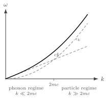
The Bogoliubov dispersion $\omega_k=\sqrt{\epsilon_k(\epsilon_k+2gn_0)}$ is linear at small $k$, with slope $c=\sqrt{gn_0/m}$, and crosses over to particle-like behavior at larger $k$. Repulsion changes the low-energy spectrum from quadratic to acoustic.

The corresponding quasiparticle operator may be written schematically as

$$b_{\mathbf k}=u_k\chi_{\mathbf k}+v_k\chi_{-\mathbf k}^\dagger, \qquad |u_k|^2-|v_k|^2=1,$$

so that the canonical commutator of $b_{\mathbf k}$ is preserved. Switching temporarily to box-normalized modes, the quadratic grand-canonical Hamiltonian for each pair $\mathbf k,-\mathbf k$ is

$$K_2=\sum_{\mathbf k\ne0}\left[ (\epsilon_k+gn_0)\chi_{\mathbf k}^\dagger\chi_{\mathbf k} +\frac{gn_0}{2} \left(\chi_{\mathbf k}^\dagger\chi_{-\mathbf k}^\dagger +\chi_{\mathbf k}\chi_{-\mathbf k}\right) \right] +\text{constant}.$$

The factor $1/2$ in the pairing term compensates for summing over both $\mathbf k$ and $-\mathbf k$. For the displayed definition of $b_{\mathbf k}$, one convenient real choice has

$$u_k^2=\frac12\left(\frac{\epsilon_k+gn_0}{\omega_k}+1\right), \qquad v_k^2=\frac12\left(\frac{\epsilon_k+gn_0}{\omega_k}-1\right),$$

with

$$u_kv_k=\frac{gn_0}{2\omega_k}.$$

Changing the sign in the definition of $b_{\mathbf k}$ changes the sign of $v_k$ and of the last equation, but not $v_k^2$ or the spectrum. This explicit relation fixes the otherwise easy-to-miss factor of two in the pairing term. At small $k$, both amplitudes are large and nearly equal: the phonon is a strongly mixed particle–hole excitation. At large $k$, $v_k\to0$ and the mode becomes particle-like.

This result is one of the simplest places where field theory improves the physical picture. A free boson at small momentum has energy $k^2/(2m)$; in the interacting condensate, trying to move one boson necessarily shakes the density and phase of the whole condensate. The low-energy object is therefore not an isolated particle but a collective wave.

Quantum depletion and control of the approximation

The quasiparticle vacuum is not the vacuum of the original particle modes. For the real coefficients used above, invert the transformation to obtain $\chi_{\mathbf k}=u_k b_{\mathbf k}-v_k b^\dagger_{-\mathbf k}$. In box normalization, its vacuum occupation is $\langle\chi^\dagger_{\mathbf k}\chi_{\mathbf k}\rangle=v_k^2$. Thus, at zero temperature, the thermodynamic-limit density outside the condensate is

$$n_{\mathrm{dep}} =\int\frac{d^3k}{(2\pi)^3}\,v_k^2 =\frac{1}{2\pi^2}\int_0^\infty dk\,k^2v_k^2.$$

The angular measure already counts all momenta; pairing $\mathbf k$ with $-\mathbf k$ adds no extra factor of two. Define $k_*=\sqrt{2mgn_0}=\xi^{-1}$ and $x=k/k_*$. Then

$$\begin{aligned} n_{\mathrm{dep}}&=\frac{(2mgn_0)^{3/2}}{2\pi^2}\,I,\\ I&=\frac12\int_0^\infty dx \left[\frac{x(x^2+1)}{\sqrt{x^2+2}}-x^2\right] =\frac{1}{3\sqrt2}. \end{aligned}$$

For example, an antiderivative of the integrand defining $I$ is

$$F(x)=\frac12\left[ \frac{(x^2+2)^{3/2}}{3}-\sqrt{x^2+2}-\frac{x^3}{3} \right].$$

Its limits are $F(0)=-1/(3\sqrt2)$ and $F(\infty)=0$. Substituting the matched $g=4\pi a/m$ gives

$$n_{\mathrm{dep}} =\frac{(mgn_0)^{3/2}}{3\pi^2} =\frac{8}{3\sqrt\pi}\,n_0\sqrt{n_0a^3}.$$

This is the leading homogeneous three-dimensional quantum-depletion result Castin 2001, arXiv v1, § 7.7, pp. 94–96, Eqs. (353)–(360), PDF. Here $n_0$ is the condensate density and the total density is $n=n_0+n_{\mathrm{dep}}$. Consequently, to the retained leading order,

$$\frac{n_{\mathrm{dep}}}{n} \simeq\frac{8}{3\sqrt\pi}\sqrt{na^3}, \qquad na^3\ll1.$$

The replacement $n_0\simeq n$ in this last expression is an order-consistent approximation, not an exact equality. Likewise the earlier mean-field normalization, $\mu=gn_0$, and the sound speed retain their leading-order meaning. For $na^3=10^{-6}$, the predicted fraction is about $0.0015045$, or $0.15045\%$: a small noncondensate population that supports the expansion about the saddle.

The contact calculation also needs a separation of scales. The characteristic momentum $k_*$ must lie below the microscopic range scale: $k_*r_0\ll1$. The effective range $r_e$ is a distinct scattering parameter; if it is anomalously large, require its correction to be small as well, for example $|a r_e|k_*^2\ll1$ in the regime $k_*a\ll1$ Castin 2001, arXiv v1, § 3.3.2, p. 33, Eq. (97), PDF. The convergent integral extended to infinite momentum yields the leading contact-limit coefficient; it is not an exact prediction of the microscopic high-momentum distribution.

Small depletion is a self-consistency test, not a bound on every observable’s error and not the superfluid fraction. Thermal populations, lower-dimensional infrared behavior, or strong depletion require a different analysis. The canonical discussion of depletion and observable response continues this distinction.

Phase and density variables

The same sound mode can be derived in a way that makes the physics more transparent. Here the polar field denotes chosen-phase mean-field or path-integral variables, not an exact operator identity involving a globally defined Hermitian phase operator. Write

$$\psi(\mathbf x,t)=\sqrt{n(\mathbf x,t)}\,e^{i\theta(\mathbf x,t)}, \qquad n(\mathbf x,t)=n_0+\delta n(\mathbf x,t),$$

where $\delta n$ is a density fluctuation. This notation avoids confusing the density fluctuation with the canonical momentum symbol used for relativistic fields later. The nonrelativistic real-time Lagrangian density in the grand-canonical frame is

$$\mathcal L_\mu =i\psi^\dagger\partial_t\psi -\frac{1}{2m}\nabla\psi^\dagger\cdot\nabla\psi +\mu\psi^\dagger\psi -\frac g2(\psi^\dagger\psi)^2.$$

After dropping total derivatives and expanding to quadratic order around $n_0=\mu/g$, one finds

$$\mathcal L^{(2)} =-\delta n\,\dot\theta -\frac{n_0}{2m}(\nabla\theta)^2 -\frac g2(\delta n)^2 -\frac{1}{8mn_0}(\nabla\delta n)^2.$$

The term $-\delta n\,\dot\theta$ says that density is conjugate to phase. At very long wavelengths the gradient term for $\delta n$ is subleading. The density fluctuation then appears algebraically, and its equation of motion is

$$\delta n=-\frac{1}{g}\dot\theta.$$

Substituting back gives the effective phase Lagrangian

$$\mathcal L_{\mathrm{eff}} =\frac{1}{2g}\dot\theta^2 -\frac{n_0}{2m}(\nabla\theta)^2.$$

The phase therefore obeys

$$\ddot\theta-c^2\nabla^2\theta=0, \qquad c^2=\frac{gn_0}{m}.$$

This derivation shows why the gapless mode is a phase oscillation, while its propagation is made possible by finite compressibility. Increasing $g$ at fixed $n_0$, while remaining in the dilute weak-coupling regime, raises the density-fluctuation cost and the leading sound velocity. If $g$ is sent to zero, the phase-only description degenerates, and one returns to the free Bose gas with quadratic excitations.

Keeping the $(\nabla\delta n)^2$ term and integrating out $\delta n$ more carefully reproduces the full Bogoliubov dispersion rather than just its small-$k$ limit. The additional $k^4$ term in $\omega_k^2$ is the remnant of the kinetic energy associated with density variation.

Landau criterion and the Mach cone

A superfluid is not merely a system with a gapless mode. A gapless mode by itself would seem to make dissipation easy. What matters is the relation between energy and momentum.

Suppose a macroscopic object moves through the condensate with momentum $\mathbf P$ and energy $E(\mathbf P)$. It can emit a collective excitation of momentum $\mathbf k$ only if energy and momentum conservation allow

$$E(\mathbf P)=E(\mathbf P-\mathbf k)+\omega(\mathbf k).$$

For a sufficiently heavy object, recoil is negligible and

$$E(\mathbf P)-E(\mathbf P-\mathbf k) =\mathbf v\cdot\mathbf k+O(k^2/M), \qquad \mathbf v=\frac{\partial E}{\partial\mathbf P}.$$

Thus the no-recoil emission threshold requires

$$\mathbf v\cdot\mathbf k\geq \omega(\mathbf k).$$

Equivalently, in the frame moving with velocity $\mathbf v$ relative to the resting fluid, an excitation has shifted energy $\omega(\mathbf k)-\mathbf v\cdot\mathbf k$. For a given excitation spectrum the intrinsic Landau critical velocity is therefore

$$\boxed{v_c=\inf_{\mathbf k\neq0}\frac{\omega(\mathbf k)}{|\mathbf k|}}.$$

For the Bogoliubov spectrum,

$$\frac{\omega_k}{k} =\sqrt{\frac{gn_0}{m}+\frac{k^2}{4m^2}},$$

so the infimum is approached as $k\to0$ and

$$v_c=c.$$

For an impurity of finite mass $M$, the recoil term is not optional. If $E(\mathbf P)=\mathbf P^2/(2M)$, exact energy conservation gives

$$\mathbf v\cdot\mathbf k =\omega_k+\frac{k^2}{2M},$$

so the one-excitation threshold is

$$v_c(M)=\inf_{k>0}\left(\frac{\omega_k}{k}+\frac{k}{2M}\right).$$

For the Bogoliubov spectrum this infimum is still $c$, approached as $k\to0$; recoil only raises the threshold at fixed nonzero $k$. For a general spectrum, the no-recoil formula is recovered as $M\to\infty$. The handwritten argument, and the Mach-cone discussion below, use that macroscopic no-recoil limit.

If $v<c$, an object moving through the condensate cannot emit a single long-wavelength phonon while conserving energy and momentum. If $v>c$, phonon emission is kinematically allowed. For the acoustic part of the spectrum, $\omega_k=ck$, the emission condition becomes

$$\mathbf v\cdot\mathbf k=ck.$$

If $\theta$ is the angle between $\mathbf v$ and the emitted phonon wavevector $\mathbf k$, then

$$\cos\theta=\frac{c}{v}.$$

This is the momentum-space version of the Mach-cone condition. The wavefront cone in real space has the complementary geometric angle, often written with $\sin\alpha=c/v$.

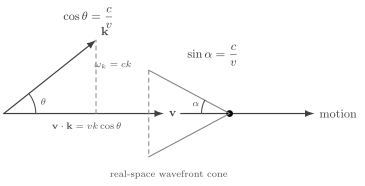
For a moving object, phonon emission requires $\mathbf v\cdot\mathbf k=\omega_k$. In the acoustic regime $\omega_k=ck$, the emitted wavevector satisfies $\cos\theta=c/v$. No such angle exists for $v<c$.

This argument is kinematic, not dynamical. It does not compute the rate of dissipation; it decides whether the simplest dissipation channel is even available. The result explains why the slope of the low-energy dispersion is so important. The linear sound mode protects the condensate from arbitrarily soft energy loss below $v_c$.

Summary

A dilute repulsive Bose gas is described at low energy by a nonlinear field equation. A coherent or selected-phase mean field, together with small depletion, supports the condensate expansion. Minimizing $H-\mu N$ gives the leading uniform condensate density

$$n_0=\frac{\mu}{g}.$$

Small fluctuations around this condensate are not ordinary free particles. Because the condensate mixes particle and hole fluctuations, the linearized equations produce the Bogoliubov spectrum

$$\omega_k=\sqrt{\epsilon_k(\epsilon_k+2gn_0)}, \qquad \epsilon_k=\frac{k^2}{2m}.$$

At small momentum this becomes sound,

$$\omega_k\simeq c k, \qquad c=\sqrt{\frac{gn_0}{m}}.$$

The same result follows from phase-density variables: density is conjugate to phase, density fluctuations encode compressibility, and the phase field is the gapless collective variable. The Landau criterion then says that the critical velocity for phonon emission is

$$v_c=\inf_{k>0}\frac{\omega_k}{k}=c$$

for this simple weakly interacting Bose condensate.

The conceptual message is bigger than this model. Field theory naturally describes collective excitations. In a condensate, the most elementary low-energy quantum is not a microscopic boson but a fluctuation of an ordered medium.

The depletion calculation quantifies the control: in the homogeneous three-dimensional zero-temperature gas, the leading noncondensate fraction is proportional to $\sqrt{na^3}$ with the matched coupling $g=4\pi a/m$. Diluteness and small range corrections are both required. Outside that regime, the formula for $\omega_k$ is no longer guaranteed, but the logic—identify the saddle, expand about it, and test the size of its fluctuations—remains one of the central moves in QFT.

Common pitfalls

1. Forgetting the chemical potential. The condensate is static only in the grand-canonical frame $K=H-\mu N$. With $H$ alone, the condensate phase rotates as $e^{-i\mu t}$.

2. Dropping the conjugate fluctuation. Linearizing with $\chi$ but not $\chi^\dagger$ misses the particle–hole mixing that produces the Bogoliubov spectrum.

3. Inferring a mean field from occupation alone. The operator $\psi$ is quantum, and a fixed-number state has $\langle\psi\rangle=0$ even with macroscopic occupation. The function $\Psi=\langle\psi\rangle$ belongs to a coherent or selected-phase description; the depletion calculation supplies a separate small-fluctuation check.

4. Treating the delta interaction as microscopic in three dimensions. The contact coupling $g$ is an effective low-energy parameter. It should not be used blindly at arbitrarily high momenta.

5. Thinking that any gapless mode guarantees superfluidity. The Landau criterion depends on the ratio $\omega(k)/k$, not just on whether $\omega(k)$ vanishes at $k=0$.

Exercises

Exercise 1

Starting from

$$H_{\mathrm{int}} =\frac12\int d^3x\,d^3y\,V(\mathbf x-\mathbf y) \psi^\dagger(\mathbf x)\psi^\dagger(\mathbf y) \psi(\mathbf y)\psi(\mathbf x),$$

show that

$$[\psi(\mathbf z),H_{\mathrm{int}}] =\int d^3y\,V(\mathbf z-\mathbf y) \psi^\dagger(\mathbf y)\psi(\mathbf y)\psi(\mathbf z),$$

assuming $V(\mathbf x-\mathbf y)=V(\mathbf y-\mathbf x)$.

Solution

Use

$$[\psi(\mathbf z),\psi^\dagger(\mathbf x)]=\delta^{(3)}(\mathbf z-\mathbf x), \qquad [\psi(\mathbf z),\psi(\mathbf x)]=0.$$

Then

$$\begin{aligned} [\psi(\mathbf z),&\psi^\dagger(\mathbf x)\psi^\dagger(\mathbf y) \psi(\mathbf y)\psi(\mathbf x)] \\ &=\delta^{(3)}(\mathbf z-\mathbf x) \psi^\dagger(\mathbf y)\psi(\mathbf y)\psi(\mathbf x) +\delta^{(3)}(\mathbf z-\mathbf y) \psi^\dagger(\mathbf x)\psi(\mathbf y)\psi(\mathbf x). \end{aligned}$$

Substituting into $H_{\mathrm{int}}$ gives two terms:

$$\frac12\int d^3y\,V(\mathbf z-\mathbf y) \psi^\dagger(\mathbf y)\psi(\mathbf y)\psi(\mathbf z)$$

and

$$\frac12\int d^3x\,V(\mathbf x-\mathbf z) \psi^\dagger(\mathbf x)\psi(\mathbf z)\psi(\mathbf x).$$

Because bosonic annihilation fields commute with one another, $\psi(\mathbf z)\psi(\mathbf x)=\psi(\mathbf x)\psi(\mathbf z)$. Renaming $\mathbf x$ as $\mathbf y$ and using the symmetry of $V$, the two terms are equal. Their sum is

$$[\psi(\mathbf z),H_{\mathrm{int}}] =\int d^3y\,V(\mathbf z-\mathbf y) \psi^\dagger(\mathbf y)\psi(\mathbf y)\psi(\mathbf z).$$

For $V(\mathbf x-\mathbf y)=g\delta^{(3)}(\mathbf x-\mathbf y)$ this becomes $g\psi^\dagger(\mathbf z)\psi(\mathbf z)\psi(\mathbf z)$.

Exercise 2

For $\mathbf k\ne0$, diagonalize the linearized Bogoliubov matrix

$$M_k= \begin{pmatrix} \epsilon_k+gn_0 & gn_0 \\ -gn_0 & -\epsilon_k-gn_0 \end{pmatrix}$$

and show that its eigenvalues are $\omega=\pm\sqrt{\epsilon_k(\epsilon_k+2gn_0)}$.

Solution

Let

$$A=\epsilon_k+gn_0, \qquad B=gn_0.$$

Then

$$M_k= \begin{pmatrix} A & B \\ -B & -A \end{pmatrix}.$$

The characteristic equation is

$$0=\det(M_k-\omega I) =\det\begin{pmatrix} A-\omega & B \\ -B & -A-\omega \end{pmatrix}.$$

Thus

$$0=(A-\omega)(-A-\omega)+B^2 =\omega^2-A^2+B^2.$$

Therefore

$$\omega^2=A^2-B^2 =(\epsilon_k+gn_0)^2-(gn_0)^2 =\epsilon_k^2+2gn_0\epsilon_k.$$

Hence

$$\omega=\pm\sqrt{\epsilon_k(\epsilon_k+2gn_0)}.$$

The positive branch is the physical excitation energy.

Exercise 3

Use the phase-density quadratic Lagrangian

$$\mathcal L^{(2)} =-\delta n\,\dot\theta -\frac{n_0}{2m}(\nabla\theta)^2 -\frac g2(\delta n)^2$$

and integrate out $\delta n$. Derive the sound velocity.

Solution

The equation of motion for $\delta n$ is

$$\frac{\partial\mathcal L^{(2)}}{\partial(\delta n)}=0 \quad\Rightarrow\quad -\dot\theta-g\delta n=0.$$

So

$$\delta n=-\frac{1}{g}\dot\theta.$$

Substitute this back:

$$-\delta n\,\dot\theta-\frac g2(\delta n)^2 =\frac{1}{g}\dot\theta^2-\frac{1}{2g}\dot\theta^2 =\frac{1}{2g}\dot\theta^2.$$

Therefore

$$\mathcal L_{\mathrm{eff}} =\frac{1}{2g}\dot\theta^2 -\frac{n_0}{2m}(\nabla\theta)^2.$$

The Euler–Lagrange equation is

$$\frac1g\ddot\theta-\frac{n_0}{m}\nabla^2\theta=0.$$

Thus

$$\ddot\theta-c^2\nabla^2\theta=0, \qquad c^2=\frac{gn_0}{m}.$$

Exercise 4

For the Bogoliubov dispersion, show directly that the Landau critical velocity is $c$.

Solution

The Landau critical velocity is

$$v_c=\inf_{k>0}\frac{\omega_k}{k}.$$

Using

$$\omega_k^2=\epsilon_k(\epsilon_k+2gn_0), \qquad \epsilon_k=\frac{k^2}{2m},$$

we find

$$\left(\frac{\omega_k}{k}\right)^2 =\frac{1}{k^2}\left(\frac{k^2}{2m}\right) \left(\frac{k^2}{2m}+2gn_0\right) =\frac{k^2}{4m^2}+\frac{gn_0}{m}.$$

This is minimized as $k\to0$, so

$$v_c=\sqrt{\frac{gn_0}{m}}=c.$$

References

• Yvan Castin, Bose-Einstein condensates in atomic gases: simple theoretical results. Lecture notes, manuscript dated 25 October 2000; arXiv:cond-mat/0105058v1 (2001). arXiv. Open PDF.

Further reading

• C. J. Pethick and H. Smith, Bose–Einstein Condensation in Dilute Gases, 2nd ed., Cambridge University Press (2008). DOI.
• Lev Pitaevskii and Sandro Stringari, Bose–Einstein Condensation and Superfluidity, Oxford University Press (2016). DOI.