Worldlines, Worldsheets, and Reparametrization Gauge

The relativistic particle is a one-dimensional generally covariant system. The field $h(\tau)$, the einbein, makes the action insensitive to how we label points along the same curve. Varying this auxiliary field imposes a constraint. This lesson develops the corresponding worldsheet geometry first for positive Euclidean metrics, then compares its constraints with their Lorentzian form.

This page turns the same idea into a two-dimensional theory. A particle sweeps out a worldline. A string sweeps out a worldsheet. The square-root length of a worldline generalizes to the square-root area of a worldsheet, and the einbein generalizes to a worldsheet metric $g_{ab}(\xi)$. This is the passage from the Nambu–Goto action to the Polyakov action.

For the worldline, gauge fixing leaves an invariant modulus. For the worldsheet, diffeomorphisms and Weyl transformations give a locally flat conformal representative. The metric equation of motion still supplies the constraints, written in Lorentzian light-cone coordinates as

$$T_{++}=0, \qquad T_{--}=0.$$

These are the classical Virasoro constraints. They are the bridge between the geometric string picture and the two-dimensional CFT machinery developed earlier in the course.

Required background. Lesson 30 supplies the relativistic worldline action, einbein, and reparametrization symmetry used below.

Worldline gauge fixing revisited

The positive Euclidean actions below use a real flat Euclidean target $\mathbb R^D$: $\dot x^2$ and $\partial_aX\cdot\partial_bX$ contract target components with $\delta_{\mu\nu}$. The worldsheet metric is also positive definite. A Euclidean worldsheet alone would not change the inherited Lorentzian target signature; the Lorentzian comparison below continues both target and worldsheet. The string tension is denoted $\mathcal T>0$ to distinguish it from stress-tensor components.

For a relativistic particle, take a dimensionless parameter $0\leq\tau\leq1$, a smooth strictly positive einbein $h(\tau)$, and the Euclidean action

$$S[x,h] ={1\over2}\int_0^1d\tau\left({\dot x^2\over h}+m^2h\right).$$

The reparametrization symmetry is

$$x(\tau)\mapsto x_f(\tau)=x(f(\tau)), \qquad h(\tau)\mapsto h_f(\tau)=f'(\tau)h(f(\tau)),$$

where $f(0)=0$, $f(1)=1$, and $f'(\tau)>0$. The combination $h(\tau)d\tau$ is invariant in the sense that its integral is unchanged:

$$L=\int_0^1h(\tau)d\tau.$$

This number $L>0$ is the worldline proper-time modulus. With $[x]=\mathrm{mass}^{-1}$, the displayed action gives $[h]=[L]=\mathrm{mass}^{-2}$. Thus $L$ is neither target arclength nor a spacetime travel time. A reparametrization can redistribute $h(\tau)$, but it cannot change $L$.

A useful way to see the correct gauge fixing is to define a new parameter

$$s(\tau)={1\over L}\int_0^\tau h(u)du.$$

This is a passive change of coordinate: $h_s(s)ds=h(\tau)d\tau$. Its inverse is the active map $f$ in the transformation above. Since $ds/d\tau=h/L>0$, we have $s(0)=0$, $s(1)=1$, and

$$h_s(s)=L.$$

Thus an endpoint-preserving reparametrization puts every such einbein in the constant gauge

$$\dot h=0, \qquad h=L,$$

followed by an integration over $L$ in the propagator. By contrast, setting $h=1$ on the interval would also fix its dimensionful modulus in the chosen units. A weaker condition such as $\ddot h=0$ leaves a linear function $h(\tau)=a+b\tau$ and therefore does not fully fix the local reparametrization freedom. The constant-metric modulus is the one appearing in Polyakov 1987, § 9.2, p. 157, Eq. (9.24).

After fixing $h=L$, the worldline action becomes

$$S[x,L] ={1\over2}\int_0^1d\tau\left({\dot x^2\over L}+m^2L\right).$$

Equivalently, with $t=L\tau$,

$$S[x,L] ={1\over2}\int_0^Ldt\left[\left({dx\over dt}\right)^2+m^2\right].$$

This is the normalization used for the scalar heat kernel in Lesson 30; its parameter is related to the conventional Schwinger parameter by $t_{\rm Sch}=L/2$. We will keep its exact modulus measure in the propagator below. Introducing and then fixing an auxiliary metric must retain this global variable and the equations obtained by varying the metric.

From lines to surfaces

A string is an extended one-dimensional object. As it evolves, it sweeps out a two-dimensional surface. Choose coordinates $\xi^1,\xi^2$ on this surface and describe its embedding into target space by

$$X^\mu=X^\mu(\xi^1,\xi^2).$$

Assume that $X$ is a smooth immersion, so its two tangent vectors are independent. The induced metric on the surface is then positive definite:

$$h_{ab}(\xi)=\partial_aX^\mu\partial_bX_\mu =\partial_aX\cdot\partial_bX.$$

The geometric area element is

$$dA=\sqrt{\det h}\,d^2\xi,$$

so the direct area action is

$$\boxed{ S_{\rm NG}[X] =\mathcal T\int d^2\xi\,\sqrt{\det h}. }$$

This is the Nambu–Goto action. It is the worldsheet analog of the square-root length action

$$S_{\rm length}=m\int ds.$$

To see how coordinate area becomes physical area, consider the regular Euclidean immersion

$$X(u,v)=\ell_0\left(u,v,\frac{u^2+v^2}{4}\right), \qquad 0\le u,v\le1,\qquad \ell_0>0.$$

The coordinates are dimensionless and $\ell_0$ is a length. Its tangent vectors give

$$\begin{aligned} X_u&=\ell_0(1,0,u/2),& X_v&=\ell_0(0,1,v/2),\\ h&=\ell_0^2\begin{pmatrix}1+u^2/4&uv/4\\uv/4&1+v^2/4\end{pmatrix},& dA&=\ell_0^2\sqrt{1+(u^2+v^2)/4}\,du\,dv. \end{aligned}$$

In the figure, follow $P=(1/2,1/2)$ from the coordinate square to the surface. These are general coordinates: at P the two tangent lengths agree, but $X_u\cdot X_v=\ell_0^2/16\ne0$. Conformal coordinates will be considered below. The surface is shown with the parallel projection $\Pi(x,y,z)=(x-y,(x+y)/3+z)$ applied to $X/\ell_0$.

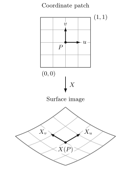
The same point P is marked in the coordinate square and its curved image. The arrows show the two coordinate directions and positive schematic multiples of $X_u$ and $X_v$, whose Gram matrix determines the induced area. The physical area scale is $\ell_0^2$; projected lengths, angles and areas are not metric measurements. This is a kinematical immersion in general coordinates, not an assumed minimal surface or classical string solution.

Editable TikZ source. Original diagram: QFT.org, created with OpenAI Codex; CC BY 4.0.

The Nambu–Goto action is manifestly geometric. It does not depend on the particular coordinates $\xi^a$ used on the surface. In the active pullback convention, take an orientation-preserving diffeomorphism of the parameter domain,

$$\xi^a\mapsto \xi'^a=f^a(\xi),$$

and transform the embedding as a scalar field on the worldsheet,

$$X^\mu(\xi)\mapsto X_f^\mu(\xi)=X^\mu(f(\xi)).$$

The induced metric transforms by pullback:

$$h_{ab}(\xi) \mapsto \partial_a f^c(\xi)\partial_b f^d(\xi)h_{cd}(f(\xi)),$$

so the transformed area density is the pullback of the original area form and its integral is unchanged. A passive relabeling uses the inverse map. If the domain has a boundary, the allowed diffeomorphisms must also preserve the boundary data. This is the two-dimensional analog of the worldline invariance of the arclength integral.

The drawback is also the same as before: the square root is awkward for quantization, and the action is nonlinear in a way that hides the relation to free two-dimensional fields. The cure is to introduce an auxiliary worldsheet metric.

The Polyakov action

The Polyakov action treats $g_{ab}(\xi)$ as an independent positive metric on the worldsheet $\Sigma$, with $g=\det g_{ab}$:

$$\boxed{ S_P[X,g] ={\mathcal T\over2}\int d^2\xi\,\sqrt g\,g^{ab}\partial_aX\cdot\partial_bX. }$$

The analogy with the worldline action is direct:

$$\text{einbein }h(\tau) \quad\longrightarrow\quad \text{worldsheet metric }g_{ab}(\xi).$$

Both are auxiliary gauge fields for reparametrization symmetry. Both make the action quadratic in derivatives of $X$. Both impose constraints when varied.

The Polyakov action has two local symmetries.

First, it is invariant under worldsheet diffeomorphisms. The embedding $X^\mu$ transforms as a scalar,

$$X^\mu(\xi)\mapsto X^\mu(f(\xi)),$$

while the metric transforms by pullback,

$$g_{ab}(\xi) \mapsto \partial_a f^c(\xi)\partial_b f^d(\xi)g_{cd}(f(\xi)).$$

Second, because the worldsheet is two-dimensional, it is invariant under Weyl rescalings

$$g_{ab}(\xi) \mapsto e^{2\omega(\xi)}g_{ab}(\xi).$$

Indeed, in two dimensions,

$$\sqrt g\mapsto e^{2\omega}\sqrt g, \qquad g^{ab}\mapsto e^{-2\omega}g^{ab},$$

so the product is invariant:

$$\sqrt g\,g^{ab} \mapsto \sqrt g\,g^{ab}.$$

This cancellation singles out strings for the kinetic action displayed here: in worldvolume dimension $n=p+1$, its density instead gains $e^{(n-2)\omega}$. It should not be mistaken for the complete auxiliary-metric area action of a higher brane. For a positive nondegenerate induced metric that action is

$$S_p={\mathcal T_p\over2}\int d^n\xi\,\sqrt g\, \bigl[g^{ab}h_{ab}-(n-2)\bigr].$$

Writing $H=g^{ab}h_{ab}$, its metric equation is $h_{ab}-\tfrac12g_{ab}[H-(n-2)]=0$. For $n\ne2$, the trace gives $H=n$, and the remaining equation gives $g_{ab}=h_{ab}$. Substitution yields $\mathcal T_p\int\sqrt h$. The additional cosmological term vanishes for a string; only then does the Weyl factor remain arbitrary. Exercise 3 concerns the kinetic density alone.

Classical equivalence to Nambu–Goto

At fixed $g$, integration by parts in the embedding variation gives both a bulk and a boundary term:

$$\begin{aligned} \delta_X S_P ={}&-\mathcal T\int_\Sigma d^2\xi\, \delta X_\mu\,\partial_a\left(\sqrt g\,g^{ab}\partial_bX^\mu\right)\\ &+\mathcal T\int_{\partial\Sigma}ds_g\, \delta X\cdot n^a\partial_aX. \end{aligned}$$

Here $n^a$ is the outward unit normal and $ds_g$ is boundary arclength. The boundary term is absent on a closed surface. It also vanishes for fixed boundary values, $\delta X=0$, or for free boundary variations with the Neumann condition $n^a\partial_aX=0$; mixed conditions apply these choices to complementary target components. With such specified conditions, the bulk equation is

$$\boxed{ \partial_a\left(\sqrt g\,g^{ab}\partial_bX^\mu\right)=0. }$$

This says that $X^\mu$ is a harmonic map from the worldsheet metric $g_{ab}$ into target space. In flat conformal gauge it will become the free Laplace or wave equation.

Now vary the inverse metric $g^{ab}$. The useful identity is

$$\delta\sqrt g=-{1\over2}\sqrt g\,g_{ab}\delta g^{ab}.$$

Therefore

$$\delta_gS_P ={\mathcal T\over2}\int d^2\xi\,\sqrt g\, \left(\partial_aX\cdot\partial_bX -{1\over2}g_{ab}g^{cd}\partial_cX\cdot\partial_dX\right)\delta g^{ab}.$$

The metric equation is the vanishing of the following constraint tensor:

$$\boxed{ \Theta_{ab} \equiv \partial_aX\cdot\partial_bX -{1\over2}g_{ab}g^{cd}\partial_cX\cdot\partial_dX =0. }$$

Thus $\delta_gS_P=(\mathcal T/2)\int\sqrt g\,\Theta_{ab}\delta g^{ab}$. The stress defined by positive covariant-metric variation is $-\mathcal T\Theta_{ab}$ with lower indices; its vanishing is the same constraint. Below, $T_{\pm\pm}$ denotes the constraint components with this overall coefficient removed, not a new normalization of the quantum CFT stress tensor.

The trace vanishes identically in two dimensions:

$$g^{ab}\Theta_{ab} =g^{ab}\partial_aX\cdot\partial_bX -{2\over2}g^{cd}\partial_cX\cdot\partial_dX =0.$$

This tracelessness is the local Noether identity associated with Weyl invariance.

To recover the Nambu–Goto action, solve the metric equation for a positive nondegenerate induced metric. It implies that $g_{ab}$ is proportional to $h_{ab}$ by a positive factor:

$$g_{ab}=e^{2\omega}h_{ab}.$$

The arbitrary Weyl factor $e^{2\omega}$ is gauge. Substituting into the Polyakov action gives

$$S_P[X,g=e^{2\omega}h] ={\mathcal T\over2}\int d^2\xi\,\sqrt h\,h^{ab}h_{ab}.$$

Since $h^{ab}h_{ab}=2$ in two dimensions,

$$S_P[X,g=e^{2\omega}h] =\mathcal T\int d^2\xi\,\sqrt h =S_{\rm NG}[X].$$

This eliminates an auxiliary metric classically, with the stated immersion and boundary assumptions. In particular, the contraction $h^{ab}h_{ab}=2$ cancels the explicit factor $1/2$ and fixes the area normalization. The metric-variation argument is developed in Polyakov 1987, § 9.5, pp. 176–177, Eqs. (9.101)–(9.108). It does not establish equality of the quantum measures for the two actions.

Reparametrization and Weyl gauge

A two-dimensional metric has three independent local components. Two diffeomorphism functions and one Weyl function suggest a local gauge choice, but function counting alone is not its proof. A smooth positive two-dimensional metric admits local isothermal coordinates in which it is conformal to a flat metric. Weyl symmetry then removes that conformal factor from the classical matter action. This is a local statement, as in Polyakov 1987, § 9.5, p. 177, Eqs. (9.109)–(9.110).

In Euclidean signature, we choose the conformal-factor convention

$$g_{ab}=e^{\phi}\delta_{ab}.$$

For the Lorentzian comparison, continue the worldsheet to signature $(+-)$ and the target to the inherited Lorentzian signature. On a local chart set $\xi^\pm=\tau\pm\sigma$. Then

$$ds^2=e^{\phi}d\xi^+d\xi^-.$$

Thus the metric components and derivatives are exactly

$$g_{++}=g_{--}=0, \qquad g_{+-}=g_{-+}={e^{\phi}\over2}, \qquad \partial_\pm={1\over2}(\partial_\tau\pm\partial_\sigma).$$

Globally, coordinate patches need not combine into one flat metric. One instead chooses conformal representatives $\widehat g_{ab}(\xi;m)$ depending on moduli $m$, and retains residual transformations that preserve the representative. These data depend on topology and on boundaries or marked points; moduli are not exclusive to higher genus. See the closed-surface discussion in Polyakov 1987, § 9.5, p. 182, Eqs. (9.141)–(9.145). On a bordered surface, preserving the boundary as a set is also different from fixing its parameterization pointwise; the disk example explicitly retains boundary reparametrization data in Polyakov 1987, § 9.5, pp. 183–184, Eqs. (9.146)–(9.155).

In conformal gauge, the Weyl factor cancels out of the classical matter action:

$$\sqrt g\,g^{ab}=\delta^{ab}$$

in Euclidean notation. Hence

$$\boxed{ S_P ={\mathcal T\over2}\int d^2\xi\,\partial_aX\cdot\partial_aX. }$$

The equation of motion becomes

$$\partial^2X^\mu=0.$$

In Lorentzian light-cone coordinates this is

$$\partial_+\partial_-X^\mu=0,$$

with the general local solution

$$X^\mu(\xi^+,\xi^-)=X_L^\mu(\xi^+)+X_R^\mu(\xi^-).$$

The gauge-fixed embedding looks like a collection of free massless scalar fields on the worldsheet. That statement is true but incomplete: the stress-tensor constraints must still be imposed.

Conformal gauge and Virasoro constraints

Gauge fixing simplifies the action, but it does not erase the metric equation of motion. The equations

$$\Theta_{ab}=0$$

survive as constraints on the free fields $X^\mu$.

In conformal light-cone coordinates, these constraints become

$$\boxed{ T_{++}=\partial_+X\cdot\partial_+X=0, \qquad T_{--}=\partial_-X\cdot\partial_-X=0. }$$

These are the Lorentzian classical Virasoro constraints. The target contraction here is Lorentzian: if the target remained positive Euclidean, the real null conditions would force both $\partial_+X$ and $\partial_-X$ to vanish. Returning to the Euclidean target and worldsheet, define $z=\xi^1+i\xi^2$, $\partial=\partial_z=(\partial_1-i\partial_2)/2$ and $\bar\partial=\partial_{\bar z}$. The classical CFT stress components are proportional to

$$T_{\mathrm{cl}}(z)\propto-\partial X\cdot\partial X, \qquad \bar T_{\mathrm{cl}}(\bar z)\propto-\bar\partial X\cdot\bar\partial X,$$

where only their zero is needed here; the quantum CFT normalization is fixed separately by the action and OPE. The classical constraints are

$$T_{\mathrm{cl}}(z)=0, \qquad \bar T_{\mathrm{cl}}(\bar z)=0.$$

After quantization these composite fields must be normal ordered, and the matter stress tensor must be combined with the ghost contribution in the BRST constraints.

In the Lorentzian chart, the equations of motion make the constraint components chiral. For example,

$$\partial_-T_{++} =2\partial_+X\cdot\partial_-\partial_+X =0,$$

and similarly

$$\partial_+T_{--}=0.$$

This is exactly the holomorphic stress-tensor structure encountered earlier in two-dimensional CFT. The difference is interpretational: in ordinary CFT the stress tensor generates conformal transformations as a global or local symmetry of correlation functions; in the Polyakov string it also enforces a gauge constraint. Physical states must satisfy the quantum version of these constraints.

A useful Euclidean way to read the conditions uses the shorthand

$$\partial_+=\partial_1-i\partial_2, \qquad \partial_-\equiv\partial_1+i\partial_2,$$

so that $\partial_+=2\partial_z$ and $\partial_-=2\partial_{\bar z}$ in this paragraph and Exercise 6. These are complex derivatives, distinct from the real Lorentzian light-cone derivatives above. Then

$$(\partial_+X)^2=0$$

is equivalent to the pair of real conditions

$$(\partial_1X)^2=(\partial_2X)^2, \qquad \partial_1X\cdot\partial_2X=0.$$

For a real Euclidean immersion, the two coordinate tangent vectors therefore have equal nonzero length and are orthogonal. The constraints make the induced metric proportional to the flat metric. Together with the harmonic equation they give a conformal minimal immersion, meaning a stationary area surface with vanishing mean curvature; they do not prove a global area minimum.

This statement also requires compatible global data. On a compact connected boundaryless worldsheet, a smooth single-valued harmonic map into $\mathbb R^D$ satisfies $\int_\Sigma\sqrt g\,|\nabla X^\mu|^2=0$ by integration by parts, hence is constant. The closed-surface variation above does not assert the existence of a nondegenerate immersion with those additional hypotheses.

The path-integral viewpoint

For target dimension $D$ and $m>0$, use the normalized Euclidean free heat kernel from Lesson 30,

$$K_L(x,y)=(2\pi L)^{-D/2} \exp\!\left[-{|x-y|^2\over2L}\right].$$

It obeys $\partial_LK_L=\tfrac12\Delta_xK_L$ and tends to $\delta^{(D)}(x-y)$ as $L\downarrow0$. Therefore the inverse kernel of $-\Delta+m^2$ is

$$\begin{aligned} G_E(x,y) &={1\over2}\int_0^\infty dL\,e^{-m^2L/2}K_L(x,y),\\ \widetilde G_E(k) &={1\over2}\int_0^\infty dL\,e^{-L(k^2+m^2)/2} ={1\over k^2+m^2}. \end{aligned}$$

The first equality is understood as a distribution when the coincident kernel is singular. Here $k$ is a real Euclidean Fourier momentum; it is not the real momentum of a classical Euclidean saddle. The kinetic path integral normalized to $K_L$ uses the action $\tfrac12\int_0^Ldt\,(dX/dt)^2$, and the mass term supplies $e^{-m^2L/2}$. Thus its exact modulus measure is $dL/2$, consistent with $t_{\rm Sch}=L/2$ and the inverse denominator in Polyakov 1987, § 9.2, p. 163, Eq. (9.46).

For strings, the corresponding object is a sum over embeddings and worldsheet geometries:

$$Z =\int {\mathcal DX\,\mathcal Dg\over \operatorname{Vol}(\operatorname{Diff}\times\operatorname{Weyl})} \,e^{-S_P[X,g]}.$$

This formula should be read with care. The division by the gauge volume is schematic; a proper quantum treatment requires gauge fixing, Faddeev–Popov ghosts, an integral over moduli, and cancellation or explicit treatment of the Weyl anomaly. But the structure is already visible:

$$\text{particle propagator}: \sum_{\text{paths}}, \qquad \text{string amplitude}: \sum_{\text{surfaces}}.$$

The next page begins to unpack this formula. Once $g_{ab}$ is treated as a dynamical integration variable, the theory resembles two-dimensional gravity coupled to matter. The conformal factor that disappeared classically can reappear through the quantum measure as a conformal anomaly, leading toward Liouville theory and nonlocal effective actions.

Summary

The worldline action

$$S[x,h]={1\over2}\int d\tau\left({\dot x^2\over h}+m^2h\right)$$

teaches the first lesson: the metric on parameter space is gauge, but gauge fixing must leave global moduli such as

$$L=\int h\,d\tau.$$

The worldsheet generalization begins with the induced metric

$$h_{ab}=\partial_aX\cdot\partial_bX$$

and the Nambu–Goto area action

$$S_{\rm NG}=\mathcal T\int d^2\xi\sqrt{\det h}.$$

Introducing an independent worldsheet metric gives the Polyakov action

$$S_P={\mathcal T\over2}\int d^2\xi\sqrt g\,g^{ab}\partial_aX\cdot\partial_bX.$$

Varying $g_{ab}$ gives the stress-tensor constraint

$$\Theta_{ab}=0,$$

which, for a positive nondegenerate induced metric, classically makes $g_{ab}$ proportional to it and recovers the Nambu–Goto action. In local Euclidean conformal gauge the action becomes a free scalar theory,

$$S_P={\mathcal T\over2}\int d^2\xi\,\partial_aX\cdot\partial_aX,$$

but the metric equation survives, with the Lorentzian comparison written as

$$T_{++}=0, \qquad T_{--}=0.$$

These are the classical Virasoro constraints, and they are the point where worldsheet geometry meets two-dimensional conformal field theory.

Common pitfalls

Do not set $h=1$ on a finite worldline interval unless the proper-time modulus has already been handled. The invariant quantity $L=\int h d\tau$ must still be integrated over.

Do not confuse the induced metric $h_{ab}=\partial_aX\cdot\partial_bX$ with the independent Polyakov metric $g_{ab}$. They become proportional only after using the $g_{ab}$ equation of motion.

Do not gauge-fix the Polyakov action and then forget the metric equation. Conformal gauge makes $X^\mu$ look free, but the constraints $T_{++}=T_{--}=0$ are still part of the theory.

Do not treat Weyl symmetry as available for every extended object. The cancellation $\sqrt g\,g^{ab}\mapsto\sqrt g\,g^{ab}$ works only in two worldsheet dimensions for this action.

Do not promote the classical equations $T_{++}=T_{--}=0$ directly to operator identities for the matter CFT. Quantum string constraints are imposed on physical states through the total matter-plus-ghost stress tensor, with anomaly cancellation required for consistency.

Exercises

Exercise 1: Constant-einbein gauge and the modulus

Show that any smooth strictly positive einbein $h(\tau)$ on $0\le \tau\le1$ can be brought to the constant value $L=\int_0^1h(\tau)d\tau$ by an endpoint-preserving reparametrization. Use a passive coordinate $s$ as above; its inverse gives the active map.

Solution

Define

$$s(\tau)={1\over L}\int_0^\tau h(u)du, \qquad L=\int_0^1h(u)du.$$

Since $h>0$, the function $s(\tau)$ is monotone, with $s(0)=0$ and $s(1)=1$. The invariant line element is

$$h(\tau)d\tau=h_s(s)ds.$$

But

$$ds={h(\tau)\over L}d\tau.$$

Therefore

$$h_s(s)=L.$$

Thus the local shape of $h(\tau)$ can be gauged away, but the constant $L$ remains.

Exercise 2: Pullback of the induced metric

For a smooth orientation-preserving diffeomorphism $f$ of the parameter domain, use the active convention $X_f=X\circ f$ to show that the induced metric

$$h_{ab}=\partial_aX\cdot\partial_bX$$

transforms by pullback.

Solution

The transformed embedding is

$$X_f^\mu(\xi)=X^\mu(f(\xi)).$$

By the chain rule,

$$\partial_aX_f^\mu(\xi) =\partial_a f^c(\xi)\partial_cX^\mu(f(\xi)).$$

Therefore

$$h^{(f)}_{ab}(\xi) =\partial_aX_f\cdot\partial_bX_f =\partial_a f^c\partial_b f^d\, \partial_cX(f(\xi))\cdot\partial_dX(f(\xi)).$$

Thus

$$h^{(f)}_{ab}(\xi) =\partial_a f^c(\xi)\partial_b f^d(\xi)h_{cd}(f(\xi)),$$

which is the pullback transformation law for a metric.

Exercise 3: Why Weyl invariance selects worldsheets

Show that the kinetic action

$$S_P={\mathcal T\over2}\int d^n\xi\sqrt g\,g^{ab}\partial_aX\cdot\partial_bX$$

is Weyl invariant for arbitrary embeddings only when the worldvolume dimension is $n=2$. This question concerns precisely the displayed kinetic action, without the cosmological term of the full higher-brane auxiliary action.

Solution

Under

$$g_{ab}\mapsto e^{2\omega}g_{ab},$$

the determinant transforms as

$$\sqrt g\mapsto e^{n\omega}\sqrt g,$$

while the inverse metric transforms as

$$g^{ab}\mapsto e^{-2\omega}g^{ab}.$$

Therefore

$$\sqrt g\,g^{ab} \mapsto e^{(n-2)\omega}\sqrt g\,g^{ab}.$$

The action is invariant for arbitrary local $\omega(\xi)$ only if

$$n-2=0,$$

so $n=2$. A string has a two-dimensional worldsheet, so the Polyakov action has Weyl symmetry. A generic $p$-brane has $n=p+1$, and this simple Weyl symmetry is absent unless $p=1$.

Exercise 4: Stress tensor from metric variation

For a positive two-dimensional auxiliary metric, derive the constraint $\Theta_{ab}=0$ from variation of the Polyakov action with respect to $g^{ab}$, using the definition $\delta_gS_P=(\mathcal T/2)\int\sqrt g\,\Theta_{ab}\delta g^{ab}$.

Solution

Start from

$$S_P={\mathcal T\over2}\int d^2\xi\sqrt g\,g^{ab}\partial_aX\cdot\partial_bX.$$

Use

$$\delta\sqrt g=-{1\over2}\sqrt g\,g_{ab}\delta g^{ab}.$$

Then

$$\delta S_P ={\mathcal T\over2}\int d^2\xi\sqrt g\, \left[ \partial_aX\cdot\partial_bX -{1\over2}g_{ab}g^{cd}\partial_cX\cdot\partial_dX \right]\delta g^{ab}.$$

Since $\delta g^{ab}$ is arbitrary, the metric equation of motion is

$$\partial_aX\cdot\partial_bX -{1\over2}g_{ab}g^{cd}\partial_cX\cdot\partial_dX=0.$$

This is the vanishing of the worldsheet stress tensor, up to the conventional overall sign and factor used in defining $T_{ab}$.

Exercise 5: Chiral conservation of the constraints

In the local Lorentzian chart $\xi^\pm=\tau\pm\sigma$, with $\partial_\pm=(\partial_\tau\pm\partial_\sigma)/2$ and Lorentzian target contraction, use $\partial_+\partial_-X=0$ to show that the constraint component $T_{++}=\partial_+X\cdot\partial_+X$ is left-moving.

Solution

Compute

$$\partial_-T_{++} =\partial_-\left(\partial_+X\cdot\partial_+X\right).$$

Using the product rule,

$$\partial_-T_{++} =2\partial_+X\cdot\partial_-\partial_+X.$$

The conformal-gauge equation of motion is

$$\partial_+\partial_-X=0.$$

Hence

$$\partial_-T_{++}=0.$$

So $T_{++}$ depends only on $\xi^+$ locally. Similarly,

$$\partial_+T_{--}=0.$$

These are the classical chiral conservation equations for the two components of the worldsheet stress tensor.

Exercise 6: Geometry of the Virasoro constraint

For a smooth real immersion into the Euclidean target, use the Euclidean definitions

$$\partial_+=\partial_1-i\partial_2, \qquad \partial_- =\partial_1+i\partial_2$$

so $\partial_+=2\partial_z$ and $\partial_-=2\partial_{\bar z}$, distinct from Exercise 5. Show that $(\partial_+X)^2=0$ is equivalent to

$$(\partial_1X)^2=(\partial_2X)^2, \qquad \partial_1X\cdot\partial_2X=0.$$

Solution

Expand

$$(\partial_+X)^2 =(\partial_1X-i\partial_2X)\cdot(\partial_1X-i\partial_2X).$$

This gives

$$(\partial_+X)^2 =(\partial_1X)^2-(\partial_2X)^2 -2i\,\partial_1X\cdot\partial_2X.$$

For this complex quantity to vanish, both its real and imaginary parts must vanish:

$$(\partial_1X)^2-(\partial_2X)^2=0,$$

and

$$\partial_1X\cdot\partial_2X=0.$$

Thus the coordinate tangent vectors have equal length and are orthogonal, which is exactly the statement that the induced metric is conformally flat in these coordinates.

References

• Polyakov, A. M. Gauge Fields and Strings. Contemporary Concepts in Physics, Vol. 3. Harwood Academic Publishers, 1987. DOI: 10.1201/9780203755082.