Wilson Loops, Worldlines, Monopole Plasma, and Confinement

A Wilson loop tests the energy needed to separate a specified external charge and anticharge. In a zero-temperature theory, a long rectangular loop projects onto the static-source spectrum. Its area term measures a string tension, provided the probes cannot be screened and the loop overlaps the relevant ground state.

This lesson connects that observable to two calculations: the leading surface term in a compact lattice theory, and the monopole-induced wall in a controlled three-dimensional Abelian effective theory. In the latter, allowed magnetic events with nonzero fugacity generate both a dual-photon mass and an electric string tension. Compactness alone does not establish those dynamical conclusions.

Required background. Compact gauge fields, Higgsing, solitons, and topological defects supplies compact connections, allowed probes and quantized magnetic flux.

Helpful background. Worldlines, worldsheets, and reparametrization gauge supplies the normalized proper-time particle kernel.

Wilson lines and charged worldlines

We use Euclidean signature. For the Abelian formulas, $A$ is the connection-normalized field: it is the preceding lesson’s $a=eA_{\rm canonical}$. A genuine compact-$U(1)$ probe has integer charge $q$, and the Maxwell action is

$$S_E[A]=\frac{1}{4e^2}\int d^D x\,F_{\mu\nu}F_{\mu\nu}, \qquad F=dA$$

locally away from magnetic insertions. The worldline interaction and its weight are

$$S_{E,\mathrm{int}}=-iq\int_C A, \qquad e^{-S_{E,\mathrm{int}}}=e^{iq\int_C A}.$$

For an open path from $y$ to $x$, the endpoint transformation is

$$U_C(x,y)\equiv e^{iq\int_y^x A} \longmapsto e^{iq\alpha(x)}U_C(x,y)e^{-iq\alpha(y)}.$$

Consequently $\psi^\dagger(x)U_C(x,y)\psi(y)$ is gauge invariant. For a closed curve the endpoint phases cancel, giving

$$W_q(C)=\left\langle e^{iq\oint_C A}\right\rangle.$$

The line integral notation includes patch transition functions when the connection is not globally a one-form. Quantized flux makes exponentiated holonomy independent of the chosen Stokes surface; it does not identify distinct Chern sectors or make every real surface integral equal.

For comparison, with a canonically normalized non-Abelian gauge field and a genuine representation $R$ of the specified global gauge group,

$$W_R(C)=\left\langle\frac{1}{\dim R}\operatorname{tr}_R \mathcal P\exp\!\left(ig\oint_C A_\mu^aT_R^a\,dx^\mu\right)\right\rangle.$$

Path ordering and the coupling $g$ are essential. The following explicit calculations use Abelian probes.

The normalized proper-time kernel

For a scalar of mass $m>0$ in a fixed smooth real background, let $D_{A,\mu}=\partial_\mu-iqA_\mu$. Its Euclidean inverse kernel is

$$\begin{aligned} G_A(x,y)&=\langle x|(-D_A^2+m^2)^{-1}|y\rangle\\ &=\int_0^\infty d\tau\,e^{-m^2\tau} \int_{X(0)=y}^{X(\tau)=x}\!\mathcal D X\, \exp\!\left[-\int_0^\tau ds\,\frac{\dot X^2}{4} +iq\int_X A\right]. \end{aligned}$$

The path measure is normalized so that its free endpoint kernel is

$$K_0(x,y;\tau)=(4\pi\tau)^{-D/2} \exp\!\left[-\frac{(x-y)^2}{4\tau}\right].$$

Here $\tau$ has dimension length squared, and the line integral uses midpoint, equivalently Stratonovich, evaluation on the Brownian path. The worldline lesson’s modulus is $L=2\tau$, so its measure $dL/2$ is precisely $d\tau$; see Polyakov 1987, § 9.2, p. 163, Eq. (9.46).

The classical expression $m\int ds\sqrt{\dot X^2}-iq\int_X A$ describes the einbein saddle. It does not assign a finite arclength to a typical Brownian path, and a charged saddle in a generic real Euclidean background can be complex. The formula above is a fixed-background propagator, before any dynamical photon or matter-loop average.

Rectangular loops and static energy

A rectangle of spatial width $R$ and Euclidean duration $T$ creates a static charge–anticharge pair, propagates it, then annihilates it. Work first at a fixed regulator in a zero-temperature theory with a positive transfer operator. With source-creating and source-annihilating operators that are adjoints, its spectral decomposition has nonnegative weights:

$$W_{\rm reg}(R,T)=\sum_n c_n(R)e^{-T V_{n,\rm reg}(R)}, \qquad c_n(R)\geq0.$$

The energies are measured relative to the vacuum. For a discrete lowest level with $c_0(R)>0$,

$$V_{0,\rm reg}(R)=-\lim_{T\to\infty}\frac{1}{T}\log W_{\rm reg}(R,T).$$

This is a matrix element with overlaps, not a thermal trace with level multiplicities. The transfer-operator relation and squared-overlap form are explicit in Bali et al. 2005, arXiv v2, § II, pp. 3–4, Eq. (13), and § III.D, pp. 13–14, Eq. (58), PDF.

Subtract the static self-energy once: define $V(R)=V_{0,\rm reg}(R)-2\delta m$ in a chosen prescription, or extract it from the correspondingly renormalized loop. The subtraction changes an additive constant, not a string tension. Spatial endpoint factors disappear after division by $T$; temporal perimeter terms shift the extracted energy.

Take $T\to\infty$ at fixed $R$ before testing large $R$, with enough spatial volume for the probes. The first relative excited-state term is $(c_1/c_0)e^{-T(V_1-V_0)}$. A tiny ground-state overlap can therefore conceal string breaking at accessible $T$; if the overlap vanishes, this operator selects the lowest state in its own spectral support. The practical obstruction is illustrated in Bali et al. 2005, arXiv v2, § V.C, p. 21, PDF.

An unscreened large-$R$ potential $V(R)=\sigma R+o(R)$ gives a leading rectangular area cost $\sigma RT$. The string tension $\sigma$ is energy per length. A perimeter contribution alone does not identify a phase: Coulomb interactions, static self-energies and screening must be distinguished by the remaining $R$ dependence.

Gaussian loops and the sign of the Coulomb potential

In noncompact Gaussian Maxwell theory, define

$$J_\mu(x)=q\oint_C dX_\mu\,\delta^{(D)}(x-X), \qquad \langle A_\mu(x)A_\nu(y)\rangle_0=e^2D_{\mu\nu}(x-y).$$

The propagator $D_{\mu\nu}$ here does not include $e^2$. Since $\partial_\mu J_\mu=0$, longitudinal gauge terms drop out of

$$W_q(C)=\exp\!\left[-\frac{e^2}{2} \int d^D x\,d^D y\,J_\mu(x)D_{\mu\nu}(x-y)J_\nu(y)\right].$$

For a smooth closed heavy-probe path, nearby segments produce a local perimeter or mass counterterm. Corners and open endpoints require additional renormalization data. The same regulated Gaussian gives the interaction between separated temporal segments.

The two long sides of a rectangle carry opposite currents. In $d_s=D-1$ spatial dimensions, their time-independent contribution is

$$\begin{aligned} V_{\rm reg}(R)&=q^2e^2[G_{\rm reg}(0)-G_{\rm reg}(R)],\\ G_{\rm reg}(R)&=\int_{\rm reg}\frac{d^{d_s}k}{(2\pi)^{d_s}} \frac{e^{i\mathbf k\cdot\mathbf R}}{\mathbf k^2}. \end{aligned}$$

The combination is ultraviolet divergent for $d_s\geq2$ until the static self-energy is treated. In low dimensions an infrared prescription is also needed for $G$ individually; potential differences remove that ambiguity. The resulting separation dependence is

$$\begin{array}{c|c} d_s&\text{charge–anticharge potential}\\ \hline 1&V(R)-V(0)=q^2e^2R/2\\ 2&V(R)-V(R_0)=q^2e^2\log(R/R_0)/(2\pi)\\ 3&V(R)=-q^2e^2/(4\pi R)+\text{constant}. \end{array}$$

The negative $1/R$ term is attraction, not a choice left open after specifying a charge–anticharge pair. In one spatial dimension, the site’s source convention gives $\partial_xE=-e^2q[\delta(x)-\delta(x-R)]$, hence $E=-e^2q$ between the probes. Its energy $\int dx\,E^2/(2e^2)=q^2e^2R/2$ explains the linear potential without monopoles. Dimension and mechanism matter.

The leading strong-coupling surface term

Consider a pure compact-$U(1)$ lattice theory at fixed spacing $a$, with one reference orientation per link and plaquette:

$$S=-\beta\sum_p\cos F_p, \qquad F_p=\sum_\ell\epsilon_{p\ell}A_\ell, \qquad A_\ell\sim A_\ell+2\pi.$$

For a positive unit Wilson insertion, write its oriented link current as $J_\ell$. Expanding the two exponentials in $e^{(\beta/2)(e^{iF}+e^{-iF})}$ gives

$$e^{\beta\cos F}=\sum_{n\in\mathbb Z}I_n(\beta)e^{inF}, \qquad I_n(\beta)=\sum_{j\geq0}\frac{(\beta/2)^{2j+|n|}}{j!(j+|n|)!}.$$

On a finite lattice this expansion is absolutely convergent. Haar integration of each link gives the exact constraint

$$\int_{-\pi}^{\pi}\frac{dA_\ell}{2\pi} e^{iA_\ell(J_\ell+\sum_p\epsilon_{p\ell}n_p)} =\delta_{J_\ell+\sum_p\epsilon_{p\ell}n_p,0}.$$

Thus the integer plaquette sheet cancels the loop current: $\partial n=-J$. On a geometric surface oriented with $\partial\Sigma=C$, the leading integers are $n_p=-1$ relative to that orientation. Their weight is unchanged by this sign because $I_{-1}=I_1$. Wilson’s original construction uses this opposite boundary orientation; see Wilson 1974, § III, pp. 2449–2450, and § IV, pp. 2453–2455.

For a contractible planar rectangle with a unique minimal sheet of $N$ plaquettes, away from periodic wrapping, the leading sheet contribution relative to the vacuum is

$$W(C)\simeq\left[\frac{I_1(\beta)}{I_0(\beta)}\right]^N, \qquad \sigma_{\rm lead}=-\frac{1}{a^2}\log\frac{I_1(\beta)}{I_0(\beta)}.$$

Since $I_0=1+O(\beta^2)$ and $I_1=\beta/2+O(\beta^3)$, this begins as $(\beta/2)^N$, with $\sigma_{\rm lead}\sim a^{-2}\log(2/\beta)$. Other sheets supply corrections; degenerate minimal sheets supply multiplicity. This fixed-loop leading calculation exhibits an area term. Establishing it uniformly as area tends to infinity at fixed nonzero $\beta$ requires control of a connected expansion, not just the first term. Wilson discusses this nonuniformity on p. 2455. Noncontractible loops require separate global-sector data.

A controlled monopole gas in three dimensions

Now work at zero temperature in three Euclidean dimensions, with $\epsilon_{123}=+1$ and

$$B_\mu=\frac12\epsilon_{\mu\nu\rho}F_{\nu\rho}, \qquad S_E=\frac{1}{2e^2}\int d^3x\,B_\mu B_\mu.$$

Specify a compact theory in which magnetic events of flux $2\pi q_a$, $q_a=\pm1$, are allowed and have nonzero weight. Smooth curvature obeys the Bianchi identity away from their cores. The event constraint is

$$\partial_\mu B_\mu=2\pi\rho, \qquad \rho(x)=\sum_a q_a\delta^{(3)}(x-x_a).$$

The calculation needs a regulator and a core prescription of inverse length $M$. Examples are a compact lattice theory at fixed cutoff, or an appropriately matched weakly coupled massive-core completion. Additional gapless matter, a Chern–Simons term, unsaturated zero modes or a symmetry forbidding unit events change the effective theory. In a Higgs completion, both charged-vector and neutral-Higgs modes must be massive above the generated scale; the massless-Higgs limit is not photon-only.

Let $\zeta>0$ be the matched fugacity per unit event, of mass dimension three. It includes the core determinant and regulated self-energy; semiclassically $\zeta=M^3\mathcal C e^{-S_0}$, with dimensionless completion-dependent $\mathcal C$. Dilute cores require $\zeta/M^3\ll1$, and the generated mass must obey $m_D\ll M$. The leading dual-field saddle will require an additional fluctuation condition below.

After matching cores and using the Coulomb kernel only at separations greater than the core size, the gas takes the form

$$\begin{aligned} Z_{\rm gas}&=\sum_{N_+,N_-}\frac{\zeta^{N_++N_-}}{N_+!N_-!} \int_{\rm cores}\prod_a d^3x_a\,e^{-S_{\rm pair}},\\ S_{\rm pair}&=\frac{1}{K}\sum_{a<b}q_aq_bG_3(x_a-x_b), \qquad G_3(r)=\frac{1}{4\pi r}, \qquad K=\frac{e^2}{4\pi^2}. \end{aligned}$$

Like charges repel and opposite charges attract. Extending the point-charge formula to zero separation would cause a collapse; the core prescription cannot be dropped.

For definiteness use a large closed box with no net boundary flux and then its bulk limit. Total magnetic charge is zero, and the finite-volume Green function has its constant mode removed; $G_3$ above is its infinite-volume local limit. On $\mathbb R^3$, neutrality is not automatic: a net charge’s $1/r^2$ field has infrared-finite exterior action. There one must specify boundary flux or choose a neutral ensemble.

The Euclidean Gaussian and the dual photon

Introduce a real Fourier multiplier $\varphi$ for the local constraint, retaining the declared boundary and zero-mode prescription. The charged first-order weight is

$$\exp\!\left[-\int d^3x\,\frac{B^2}{2e^2} -\frac{i}{2\pi}\int d^3x\,\varphi(\partial_\mu B_\mu-2\pi\rho)\right].$$

After integration by parts, the $B$ integral is a positive Gaussian with an imaginary source:

$$\begin{aligned} -\frac{B^2}{2e^2}+\frac{i}{2\pi}B\cdot\partial\varphi &=-\frac{1}{2e^2}\left(B-\frac{ie^2}{2\pi}\partial\varphi\right)^2 -\frac{e^2}{8\pi^2}(\partial\varphi)^2,\\ e^{i\int\rho\varphi}&=\prod_a e^{iq_a\varphi(x_a)}. \end{aligned}$$

This derives $K=e^2/(4\pi^2)$ and the positive-charge vertex. It does not assert an equality between the real Euclidean fields $B$ and $e^2\partial\varphi/(2\pi)$. The Gaussian’s conditional mean is imaginary, $ie^2\partial\varphi/(2\pi)$. The local Fourier multiplier, the compact identification $\varphi\sim\varphi+2\pi$ and the global flux sum play different roles. In the closed-box ensemble, integrating the compact constant mode enforces total charge zero.

As a coefficient check, $\langle\varphi(x)\varphi(y)\rangle_0=G_3(x-y)/K$. Removing diagonal self-contractions into the fugacity gives

$$\left\langle\prod_a :e^{iq_a\varphi(x_a)}:\right\rangle_0 =\exp\!\left[-\frac{1}{2K}\sum_{a\ne b}q_aq_bG_3(x_a-x_b)\right],$$

with the same core and zero-mode restrictions. The factor $1/2$ in this double sum is necessary. The plasma-to-dual-field method is developed in Polyakov 1987, § 4, pp. 65–68; the coefficients here follow the displayed Gaussian in our unit-flux convention.

Summing the two event signs gives a cosine. After matching its ultraviolet self-contractions and local terms, the leading long-distance action is

$$S_{\rm dual}=\int d^3x\left[ \frac K2(\partial\varphi)^2+2\zeta(1-\cos\varphi)\right].$$

Here and below $\zeta$ denotes the coefficient in this matched convention. Higher harmonics and derivative operators depend on the core completion and its cluster expansion; they are not included in this leading action. Their effects at momenta of order $m_D$ must also be small in the chosen completion; core dilution alone does not ensure that condition. Expanding about a minimum gives

$$m_D^2=\frac{2\zeta}{K}=\frac{8\pi^2\zeta}{e^2}.$$

This is the leading screening mass. Rescale $y=m_Dx$ to obtain

$$S_{\rm dual}=\frac{K}{m_D}\int d^3y\, \left[\frac12(\partial_y\varphi)^2+1-\cos\varphi\right].$$

Thus infrared fluctuation corrections to the saddle are small when $m_D/K\ll1$, in addition to core dilution and scale separation. Ultraviolet self-contractions have already been matched: an unrenormalized cutoff cosine has cutoff-sensitive corrections that this infrared parameter does not bound.

The Gaussian integration also leaves a contact term in the magnetic correlator. At quadratic order in the matched dual theory, using Euclidean momentum $p$,

$$\langle B_\mu(p)B_\nu(-p)\rangle_c =e^2\left[\delta_{\mu\nu}-\frac{p_\mu p_\nu}{p^2+m_D^2}\right].$$

The momentum-conserving delta is suppressed. The first term is local; the separated-point part decays on scale $m_D^{-1}$. At zero fugacity this reduces to the transverse Maxwell covariance. Magnetic screening is not screening of external electric probes: the Wilson insertion must still be evaluated.

A Wilson loop forces a smooth dual wall

Let $\Sigma$ have the Stokes orientation $\partial\Sigma=C$. Define its normal surface distribution by

$$\eta_{\Sigma,\mu}(x)=\int_\Sigma dS_\mu(y)\,\delta^{(3)}(x-y).$$

The positive unit insertion is $\exp(i\int_\Sigma B\cdot dS)$. Repeating the same first-order Gaussian therefore replaces the gradient term by

$$\frac K2\bigl(\partial\varphi+2\pi\eta_\Sigma\bigr)^2.$$

This expression uses a common regulator, not the square of an untreated delta distribution. Across a locally flat cut with normal coordinate $z$, cancellation of the singular term requires the chosen branch to have

$$\Delta_n\varphi_{\rm cut}=-2\pi.$$

The cut is auxiliary. Define a continuous neighboring lift

$$\Phi(z)=\varphi_{\rm cut}(z)+2\pi H(z), \qquad \Phi(-\infty)=0,\qquad\Phi(+\infty)=2\pi.$$

Then $\partial_z\Phi=\partial_z\varphi_{\rm cut}+2\pi\delta(z)$ and $\cos\Phi=\cos\varphi_{\rm cut}$. The Wilson problem becomes an ordinary smooth interpolation on a real lift of the compact field. Its endpoints are the same compact value, not distinct physical vacua. Moving the arbitrary cut changes the branch description, while the resolved wall has a physical thickness and energy.

Here $H$ is the Heaviside step function. In the figure, compare the upper panel’s chosen cut with the lower panel’s continuous transverse lift: the negative branch jump cancels the singular source, while the smooth profile carries the wall energy.

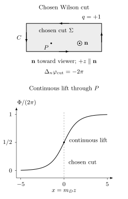
A positive unit Wilson loop fixes the Stokes orientation. Its coordinate branch jumps by $-2\pi$ along the normal; removing the cut gives the continuous lift $\Phi=4\arctan e^{m_Dz}$, from $0$ to $2\pi$ along the same normal. These endpoints are the same compact value. The upper geometry is schematic; the lower curve is the exact flat-wall profile, used locally away from the loop boundary. The arbitrary cut is placed at the smooth wall center. The finite plotted interval does not reach either asymptotic value. The leading wall tension is $\sigma_{\rm SG}=8Km_D$ under the stated probe and matching assumptions.

Editable figure source. Original QFT.org illustration, created with Codex; CC BY 4.0.

For a locally planar unit wall, the first integral with vacuum endpoints is

$$\frac K2(\Phi')^2=2\zeta(1-\cos\Phi), \qquad \Phi'=2m_D\sin\frac{\Phi}{2}.$$

The increasing solution and its tension are

$$\begin{aligned} \Phi(z)&=4\arctan e^{m_D(z-z_0)},\\ \sigma_{\rm SG}&=\int_{\mathbb R}dz\, \left[\frac K2(\Phi')^2+2\zeta(1-\cos\Phi)\right]\\ &=K\int_0^{2\pi}d\Phi\,2m_D\sin\frac{\Phi}{2} =8Km_D=\frac{2e^2m_D}{\pi^2}. \end{aligned}$$

Reversing the probe orientation reverses the lift and leaves its energy unchanged. The wall thickness is of order $m_D^{-1}$. With the displayed action fixed, the coefficient $8$ is determined; the ultraviolet completion determines the matched parameters and omitted operators.

For an unscreened unit probe, loops much larger than that thickness and a controlled local saddle give the leading wall contribution

$$-\log W_1(C)=\sigma_{\rm SG}A_{\min}(C) +\text{perimeter, fluctuation and matching corrections}.$$

For a large rectangle this yields the leading string tension in $V(R)$. Smooth-wall reasoning applies away from its boundary; rectangular corners have separate local terms. At fixed core scales, $m_D$ and $\sigma_{\rm SG}$ begin at order $e^{-S_0/2}$ times their prefactors, so the effect is absent at every finite order of ordinary perturbation theory.

This establishes a controlled infrared mechanism in the specified theory. It is not a proof of a nonzero mass gap in the strict $a\to0$ pure-lattice limit at fixed dimensional coupling. The compact monopole-plasma treatment isolates this same mechanism; the earlier course derivation develops its matching and source conventions further.

Screening and the limits of the area criterion

For genuine integer $U(1)$ probes and dynamical charges $q_i$, the screening subgroup is

$$\Lambda_{\rm screen}=\sum_i q_i\mathbb Z.$$

A probe in this subgroup can be neutralized by matter, including composites: charges $2$ and $3$ can screen a unit probe. This is the Abelian charge-lattice form of considering electric charges modulo matter charges; see Gaiotto et al. 2015, arXiv v2, § 4.2, p. 19, PDF.

When finite-energy screening clouds exist and the matter masses are finite, two separated screened probes give a trial state of bounded large-$R$ energy. An indefinitely rising string then cannot remain the ground state. Heavy matter can postpone string breaking; it need not be light. Taking its mass to infinity first instead removes that screening channel. Unscreenability alone does not prove confinement: a Coulomb phase also has unscreened probes.

For a specified $SU(N)$ theory, adjoint gluons carry zero $N$-ality and cannot screen a nonzero center charge; additional matter reduces the surviving classes. The genuine lines depend on the global gauge group. In a confining regime the asymptotic tension can depend on the remaining class, rather than the full representation. These group-theoretic constraints are not a derivation of ordinary four-dimensional Yang–Mills confinement.

In four Euclidean dimensions magnetic particles trace worldlines rather than point events, so the three-dimensional gas and scalar action cannot simply be copied. The dual-superconductor picture motivates flux tubes, but supplies no general weakly coupled proof for ordinary four-dimensional Yang–Mills here. The next lesson, strings, branes, sigma models, and AdS hints, develops the geometric language suggested by paths and surfaces.

Common pitfalls

A photon mass is not an area law. A charge-one Abelian Higgs condensate can fully screen integer probes while making the photon massive. In the monopole calculation, it is the Wilson-induced wall, not the mass alone, that establishes the leading string energy.

The cut is not a physical discontinuous wall. Its signed jump cancels the prescribed singular source. The energy is carried by the smooth continuous lift over a finite thickness.

A leading term is not a uniform limit. The first lattice sheet, finite-$T$ spectral fit and local sine-Gordon saddle each require their own control before an asymptotic confinement claim.

Exercises

Exercise 1: Rectangular Wilson loops and static potentials

At fixed $R$, suppose a zero-temperature rectangular Wilson loop has a discrete gapped expansion

$$W(R,T)=A_0(R)e^{-T V_0(R)}+A_1(R)e^{-T V_1(R)}+\cdots,$$

where $V_0(R)<V_1(R)<\cdots$, $A_n(R)\geq0$ and $A_0(R)>0$. Use a single consistent static self-energy prescription. Show that

$$V_0(R)=-\lim_{T\to\infty}{1\over T}\log W(R,T).$$

Solution

Factor out the lowest exponential:

$$W(R,T)=A_0(R)e^{-T V_0(R)} \left[1+{A_1(R)\over A_0(R)}e^{-T(V_1(R)-V_0(R))}+\cdots\right].$$

Taking the logarithm gives

$$\log W(R,T)=\log A_0(R)-T V_0(R) +\log\left[1+O(e^{-T(V_1-V_0)})\right].$$

Dividing by $-T$ and taking $T\to\infty$ removes the finite prefactor and the exponentially small corrections:

$$-\lim_{T\to\infty}{1\over T}\log W(R,T)=V_0(R).$$

Exercise 2: Linear potential in one spatial dimension

In one spatial dimension, place charges $+q$ at $x=0$ and $-q$ at $x=R$. Let the electrostatic energy be

$$E_{\rm field}={1\over2e^2}\int dx\,E^2(x),$$

and impose Gauss’s law

$$\partial_xE=-e^2q\bigl[\delta(x)-\delta(x-R)\bigr].$$

Assuming $E=0$ outside the interval $[0,R]$, find $V(R)$.

Solution

Integrating Gauss’s law across $x=0$ gives a jump $E(0^+)-E(0^-)=-e^2q$. Since $E=0$ for $x<0$, we get $E=-e^2q$ for $0<x<R$. Across $x=R$, the charge $-q$ brings the field back to zero.

Therefore

$$V(R)=E_{\rm field}={1\over2e^2}\int_0^R dx\,e^4q^2 =\frac{e^2q^2}{2}R.$$

The force is constant. This is the one-dimensional Coulomb law.

Exercise 3: The oriented strong-coupling sheet

For a contractible planar rectangular loop with a unique minimal sheet, use

$$e^{\beta\cos F_p}=\sum_{n_p\in\mathbb Z}I_{n_p}(\beta)e^{in_pF_p}$$

and the link integral

$$\int_0^{2\pi}{dA\over2\pi}e^{imA}=\delta_{m,0}$$

to obtain the leading surface contribution. Specify its orientation relative to the positive Wilson insertion, and distinguish this fixed-loop calculation from a uniform large-area conclusion.

Solution

After expanding every plaquette factor, the path integral contains products of phases

$$\exp\left(i\sum_p n_pF_p+i\sum_{\ell\in C}A_\ell\right).$$

Since each plaquette angle $F_p$ is a signed sum of link angles, the exponent can be rewritten as

$$i\sum_\ell A_\ell\left(J_\ell+\sum_p \epsilon_{p\ell}n_p\right),$$

where $J_\ell$ is the integer current supported on the Wilson loop. Integrating over each link imposes

$$J_\ell+\sum_p\epsilon_{p\ell}n_p=0.$$

Thus the integer sheet has boundary $-C$. Relative to a geometric minimal surface oriented with $\partial\Sigma=C$, choose $n_p=-1$ on its plaquettes and zero elsewhere. Since $I_{-1}=I_1$, the leading relative weight is

$$\left({I_1(\beta)\over I_0(\beta)}\right)^{N_{\min}(C)}.$$

For $\beta\ll1$, this begins as $(\beta/2)^{N_{\min}}$. With $A_{\min}^{\rm phys}=a^2N_{\min}$, its leading area coefficient is $\sigma_{\rm lead}\sim a^{-2}\log(2/\beta)$. Controlling corrections as area grows at fixed nonzero coupling requires a connected expansion; the single minimal sheet alone does not prove that uniform statement.

Exercise 4: Dual-photon mass from the monopole fugacity

Consider the matched leading sine-Gordon action with $K,\zeta>0$,

$$S=\int d^3x\left[{K\over2}(\partial\varphi)^2+2\zeta(1-\cos\varphi)\right].$$

Expand around $\varphi=0$ and find the quadratic dual-photon mass.

Solution

For small $\varphi$,

$$1-\cos\varphi={\varphi^2\over2}+O(\varphi^4).$$

Thus

$$2\zeta(1-\cos\varphi)=\zeta\varphi^2+O(\varphi^4) ={1\over2}(2\zeta)\varphi^2+O(\varphi^4).$$

The quadratic action is

$$S_2=\int d^3x\left[{K\over2}(\partial\varphi)^2+{1\over2}(2\zeta)\varphi^2\right].$$

Therefore

$$m_D^2={2\zeta\over K}.$$

With $K=e^2/(4\pi^2)$, this gives

$$m_D^2={8\pi^2\zeta\over e^2}.$$

Exercise 5: Why a smooth dual wall gives an area term

Assume the unscreened unit Wilson probe requires a continuous neighboring lift from $0$ to $2\pi$, after the auxiliary cut is removed. Let its leading sine-Gordon tension be $\sigma$. For a loop much larger than the wall thickness, explain the leading semiclassical area contribution.

Solution

The Wilson insertion fixes a winding condition on the continuous lift. Its endpoints are equivalent compact values; they are separated by a nontrivial interpolation in the specified probe sector.

For a large smooth loop, the wall thickness is microscopic compared with the loop size. The action of a wall configuration is approximately tension times area:

$$S_{\rm wall}[\Sigma]\simeq \sigma A(\Sigma).$$

At leading saddle order the least-action wall has minimal area:

$$S_{\rm saddle}\simeq \sigma A_{\min}(C).$$

Therefore the leading wall contribution is

$$W(C)\sim e^{-S_{\rm saddle}} =e^{-\sigma A_{\min}(C)}.$$

For a rectangle, $A_{\min}=RT$, so the leading term is $W(R,T)\sim e^{-\sigma RT}$ and $V(R)\sim\sigma R$. Boundary, fluctuation and matching corrections are separate from this leading saddle result.

References

• Bali, Gunnar S., Hartmut Neff, Thomas Düssel, Thomas Lippert, and Klaus Schilling (SESAM Collaboration). “Observation of String Breaking in QCD.” Physical Review D 71 (2005): 114513. DOI: 10.1103/PhysRevD.71.114513. Open PDF, arXiv v2.
• Gaiotto, Davide, Anton Kapustin, Nathan Seiberg, and Brian Willett. “Generalized Global Symmetries.” Journal of High Energy Physics 02 (2015): 172. DOI: 10.1007/JHEP02(2015)172. Open PDF, arXiv v2.
• Polyakov, A. M. Gauge Fields and Strings. Contemporary Concepts in Physics, vol. 3. Harwood Academic Publishers, 1987. DOI: 10.1201/9780203755082.
• Wilson, Kenneth G. “Confinement of Quarks.” Physical Review D 10 (1974): 2445–2459. DOI: 10.1103/PhysRevD.10.2445. Open PDF, University of Crete teaching copy.