Free Fields, Wightman Functions, and the iε Prescription

Positive energy determines which side of real time defines a vacuum correlator. Starting from a normalized free oscillator, this lesson derives Wightman functions, time ordering and the Feynman prescription, then uses scalar conformal correlators to connect boundary values with causal support. Spinful fields need an additional continuation of their frames and normalization; a physical Majorana example makes those factors explicit.

The point of this page is not merely to remember where the symbol $i\epsilon$ goes. The real lesson is analytic. A vacuum correlator such as $\langle0|\phi(t)\phi(0)|0\rangle$ is generally a distribution on the real time axis. Because the spectrum is bounded below, it is the boundary value of a function analytic in one half of the complex time plane. Different operator orderings arise from different analytic functions and different sides of approach. The familiar Feynman prescription is the compact way of keeping track of these boundary values.

This becomes especially sharp in conformal field theory. Euclidean correlators are ordinary power laws. Lorentzian correlators are distributions obtained by approaching their singular light cones from specified sides. The distinction between

$${1\over (\mathbf x^2-t^2)^\Delta}, \qquad {1\over (\mathbf x^2-(t-i0)^2)^\Delta}, \qquad {1\over (\mathbf x^2-t^2+i0)^\Delta}$$

is the distinction between a formal expression, a Wightman boundary value, and a time-ordered correlator with its coincident extension still to be specified when necessary. The free-field calculations start with a massive real scalar; massless limits and scalar primaries in a unitary conformal vacuum are treated under the stated dimension and distributional hypotheses.

Required background. Lesson 16 supplies the oscillator normalization and distinguishes conformal coordinate maps from transformations of physical fields and spin frames.

Helpful background. Lesson 15 supplies primary weights and normalized conformal two-point functions.

One oscillator already contains the prescription

Lorentzian boundary values

For Lorentzian time $t$ and spatial separation $\mathbf x$, write

$$\rho=\mathbf x^2-t^2,$$

because free and conformal scalar correlators naturally appear with denominators of the form $\mathbf x^2-(t\mp i0)^2$. The symbol $0$ means a positive infinitesimal. Thus

$$t-i0$$

means that the real time $t$ is approached from the lower half of the complex $t$-plane.

Start with a single harmonic oscillator of frequency $\omega>0$, with mechanical mass set to one as in Schwartz 2014, § 2.2.1, p. 18:

$$q(t)={1\over\sqrt{2\omega}} \left(ae^{-i\omega t}+a^\dagger e^{i\omega t}\right), \qquad [a,a^\dagger]=1, \qquad a|0\rangle=0.$$

Then

$$\begin{aligned} W_+(t) &=\langle0|q(t)q(0)|0\rangle \\ &={1\over2\omega}\langle0| \left(ae^{-i\omega t}+a^\dagger e^{i\omega t}\right)(a+a^\dagger)|0\rangle \\ &={e^{-i\omega t}\over2\omega}. \end{aligned}$$

The opposite ordering gives

$$W_-(t)=\langle0|q(0)q(t)|0\rangle ={e^{+i\omega t}\over2\omega}=W_+^*(t),$$

for real $t$. Because the oscillator commutator is a c-number, their difference is the commutator itself (times the identity operator),

$$[q(t),q(0)]=W_+(t)-W_-(t) =-{i\sin\omega t\over\omega}.$$

This calculation displays three features that survive the field-theory limit.

First, a Wightman function is not time ordered. It is an ordinary vacuum expectation value in a specified operator order.

Second, $W_+(t)$ contains only positive energies propagating forward in the chosen ordering. It oscillates as $e^{-i\omega t}$, not as a symmetric cosine.

Third, the commutator is not the same object as the Wightman function. The Wightman function knows about vacuum fluctuations. The commutator supplies the spectral kernel from which causal response is built; a retarded correlator also includes the appropriate step function and convention-dependent factor of $i$.

For a real free scalar of mass $m>0$ in $D=d+1$ spacetime dimensions, the oscillator label becomes a $d$-component spatial momentum:

$$\phi(t,\mathbf x) =\int {d^d\mathbf p\over(2\pi)^d}{1\over\sqrt{2\omega_{\mathbf p}}} \left( a_{\mathbf p}e^{-i\omega_{\mathbf p}t+i\mathbf p\cdot\mathbf x} +a_{\mathbf p}^\dagger e^{i\omega_{\mathbf p}t-i\mathbf p\cdot\mathbf x} \right),$$

where

$$\omega_{\mathbf p}=\sqrt{\mathbf p^2+m^2}, \qquad [a_{\mathbf p},a_{\mathbf q}^\dagger]=(2\pi)^d\delta^{(d)}(\mathbf p-\mathbf q).$$

The positive-frequency Wightman function is therefore

$$\boxed{ W_+(t,\mathbf x) =\langle0|\phi(t,\mathbf x)\phi(0)|0\rangle =\int {d^d\mathbf p\over(2\pi)^d}{1\over2\omega_{\mathbf p}} e^{-i\omega_{\mathbf p}t+i\mathbf p\cdot\mathbf x}. }$$

Similarly,

$$W_-(t,\mathbf x) =\langle0|\phi(0)\phi(t,\mathbf x)|0\rangle =W_+(-t,-\mathbf x).$$

For the parity-even free scalar used here—or whenever spatial inversion is a symmetry—$W_+(-t,-\mathbf x)=W_+(-t,\mathbf x)$. Ordinary rotations already imply this for $d\ge2$; in one spatial dimension parity is an additional assumption. Thus

$$W_-(t,\mathbf x)=W_+(-t,\mathbf x).$$

In momentum space the same object can be written invariantly as

$$W_+(x) =\int {d^D p\over(2\pi)^D} (2\pi)\theta(p^0)\delta(p^2-m^2)e^{-ip\cdot x}, \qquad D=d+1.$$

The step function $\theta(p^0)$ restricts $W_+$ to positive-energy on-shell modes. The massive mode expansion and ordered vacuum kernel are developed in Schwartz 2014, § 6.2, p. 75.

Spectral positivity and half-plane analyticity

The oscillator result is not an accident of free fields. Let $O(t)=O(t)^\dagger$ be a Hermitian Heisenberg operator in a theory whose Hamiltonian has an exact vacuum $|\Omega\rangle$ and a spectrum bounded below. Write $H|\Omega\rangle=E_\Omega|\Omega\rangle$.

For an operator, assume the vacuum lies in its domain. For a local field, the point notation below is distributional shorthand: use suitable smearing and a positive spectral measure of at most polynomial growth. These conditions justify exponential damping and differentiation inside the analytic half-plane; positive energies without a growth condition are not enough for an arbitrary formal series.

Insert a complete set of energy eigenstates, with the sum understood to include continuum integrals:

$$\begin{aligned} \langle\Omega|O(t)O(0)|\Omega\rangle &=\sum_n\langle\Omega|O(t)|n\rangle \langle n|O(0)|\Omega\rangle \\ &=\sum_n |\langle n|O(0)|\Omega\rangle|^2 e^{-i(E_n-E_\Omega)t}. \end{aligned}$$

For a non-Hermitian operator, the positive-type correlator is instead $\langle\Omega|O(t)O^\dagger(0)|\Omega\rangle$; its coefficients are again absolute squares. One may also replace $O$ by $O-\langle\Omega|O|\Omega\rangle$ when the vacuum contribution is not wanted.

Since $E_n-E_\Omega\ge0$, the exponential becomes

$$e^{-i(E_n-E_\Omega)(t_R+i t_I)} =e^{-i(E_n-E_\Omega)t_R}e^{(E_n-E_\Omega)t_I}.$$

The sum is damped when $t_I<0$. More explicitly, write $d\mu(E)$ for the positive spectral measure with $E=E_n-E_\Omega\ge0$. If $\mu([0,E])\le A(1+E)^N$, then $\int_0^\infty E^k e^{-aE}\,d\mu(E)<\infty$ for every $a>0$ and nonnegative integer $k$. These bounds hold uniformly on compact subsets of the lower half-plane, so differentiation under the integral proves analyticity. The positive spectral construction is discussed in Schwartz 2014, § 24.2.1, pp. 467–468; the argument here permits a zero-energy contribution and does not require a mass gap.

It defines the analytic function

$$F_+(z)=\sum_n |\langle n|O|\Omega\rangle|^2 e^{-i(E_n-E_\Omega)z}, \qquad \operatorname{Im}z<0.$$

The reversed ordering similarly comes from

$$F_-(z)=\sum_n |\langle n|O|\Omega\rangle|^2 e^{+i(E_n-E_\Omega)z}, \qquad \operatorname{Im}z>0.$$

The real-time Wightman distributions are their boundary values:

$$\boxed{ \begin{aligned} W_+(t)&:=\langle\Omega|O(t)O(0)|\Omega\rangle =\lim_{\epsilon\downarrow0}F_+(t-i\epsilon),\\ W_-(t)&:=\langle\Omega|O(0)O(t)|\Omega\rangle =\lim_{\epsilon\downarrow0}F_-(t+i\epsilon). \end{aligned} }$$

These limits are generally limits of distributions, not pointwise limits. For finite $\epsilon>0$, the first spectral sum contains the genuine damping factor $e^{-\epsilon(E_n-E_\Omega)}$. The notation $i0$ records the side from which the distributional boundary is taken after $\epsilon\downarrow0$; it is not itself a finite convergence factor.

The figure separates the analytic functions from their boundary distributions. Inspect the vertical approach arrows. The point $t_C=-i\tau$, $\tau>0$, lies inside the lower half-plane and will give the positive-time Euclidean correlator in the next section.

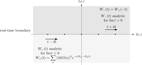
For the declared positive-type vacuum correlator and spectral growth, damping defines $F_+(t_C)$ below real time and $F_-(t_C)$ above it. Their distributional boundaries are $W_+$ and $W_-$. For the scalar, $t_C=-i\tau$ with $\tau>0$ gives the Euclidean value. The complex-time diagram is schematic; the two boundary distributions need not agree.

The finite imaginary displacement supplies spectral damping; its limiting side encodes the spectrum condition and the operator ordering.

A useful boundary-value mnemonic is:

$$\begin{array}{ccl} \langle\Omega|O(t)O(0)|\Omega\rangle &:& z\to t-i0,\\ \langle\Omega|O(0)O(t)|\Omega\rangle &:& z\to t+i0. \end{array}$$

The sign is easy to remember from damping. Positive energies $e^{-iEt}$ decay when $t$ is moved downward.

Euclidean continuation

Set

$$t=-i\tau.$$

For $\tau>0$, this lies in the lower half-plane, so the analytic function whose boundary is $W_+$ gives

$$F_+(-i\tau,\mathbf x) =\int {d^d\mathbf p\over(2\pi)^d}{1\over2\omega_{\mathbf p}} e^{-\omega_{\mathbf p}\tau+i\mathbf p\cdot\mathbf x}.$$

This is the Euclidean two-point function for positive Euclidean time separation. In fully Euclidean momentum notation,

$$G_E(\tau,\mathbf x) =\int {d^D p_E\over(2\pi)^D} {e^{ip_E^0\tau+i\mathbf p\cdot\mathbf x}\over (p_E^0)^2+\mathbf p^2+m^2}.$$

The integral over $p_E^0$ can be done by closing the contour. It gives

$$G_E(\tau,\mathbf x) =\int {d^d\mathbf p\over(2\pi)^d}{1\over2\omega_{\mathbf p}} e^{-\omega_{\mathbf p}|\tau|+i\mathbf p\cdot\mathbf x}.$$

Thus Euclidean reflection symmetry in $\tau$ packages both Wightman orderings:

$$\tau>0 \quad \leftrightarrow \quad \langle\phi(t)\phi(0)\rangle,$$

while

$$\tau<0 \quad \leftrightarrow \quad \langle\phi(0)\phi(t)\rangle.$$

For a massless scalar in $D$ Euclidean dimensions,

$$G_E(x_E)=\int {d^D p_E\over(2\pi)^D}{e^{ip_E\cdot x_E}\over p_E^2} ={\Gamma(D/2-1)\over4\pi^{D/2}} {1\over |x_E|^{D-2}}, \qquad D>2.$$

The restriction $D>2$ matters. In $D=2$ the massless scalar Green function is logarithmic rather than a power law, and the undifferentiated scalar has an infrared zero-mode subtlety. Its derivatives and suitably neutral vertex operators are the better-defined conformal observables.

This is exactly the form expected for a scalar operator of dimension

$$\Delta_\phi={D-2\over2}.$$

To obtain the first ordering, set $\tau=\epsilon+it$ with $\epsilon>0$, and only then take $\epsilon\downarrow0$. This gives

$$\boxed{ W_+(t,\mathbf x) ={\Gamma(D/2-1)\over4\pi^{D/2}} {1\over \left(\mathbf x^2-(t-i0)^2\right)^{(D-2)/2}}. }$$

For $D=4$, this reduces to

$$W_+(t,\mathbf x) ={1\over4\pi^2}{1\over \mathbf x^2-(t-i0)^2}.$$

The reversed ordering is the other boundary value:

$$W_-(t,\mathbf x) ={1\over4\pi^2}{1\over \mathbf x^2-(t+i0)^2}.$$

Time ordering and the Feynman prescription

Write the raw time-ordered two-point function as $D_F$:

$$D_F(t,\mathbf x) =\langle0|T\phi(t,\mathbf x)\phi(0)|0\rangle =\theta(t)W_+(t,\mathbf x)+\theta(-t)W_-(t,\mathbf x).$$

For the free scalar field, this equals

$$\boxed{ D_F(x)=\int {d^D p\over(2\pi)^D}{i e^{-ip\cdot x}\over p^2-m^2+i0}. }$$

For the free scalar, $(\Box+m^2)D_F=-i\delta^{(D)}$, while the delta-normalized inverse is $G_F=iD_F$. This is the same dictionary as Scalar Propagators, Ordered Correlators, and Sources. At fixed spatial momentum,

$$D_F(t,\mathbf p) =\int {dp^0\over2\pi}{i e^{-ip^0t}\over (p^0)^2-\omega_{\mathbf p}^2+i0}.$$

For a finite regulator $\epsilon>0$ and $\omega_{\mathbf p}>0$, the denominator

$$D_\epsilon(p^0)=(p^0)^2-\omega_{\mathbf p}^2+i\epsilon$$

has the exact roots

$$p^0=\pm\sqrt{\omega_{\mathbf p}^2-i\epsilon} = \begin{cases} +\omega_{\mathbf p}-i\epsilon/(2\omega_{\mathbf p}) +O(\epsilon^2/\omega_{\mathbf p}^3),\\ -\omega_{\mathbf p}+i\epsilon/(2\omega_{\mathbf p}) +O(\epsilon^2/\omega_{\mathbf p}^3). \end{cases}$$

Thus the positive-energy pole approaches the real axis from below and the negative-energy pole from above. The useful statement at the boundary is the distributional partial-fraction identity

$$\boxed{ {1\over(p^0)^2-\omega_{\mathbf p}^2+i0} ={1\over2\omega_{\mathbf p}} \left( {1\over p^0-\omega_{\mathbf p}+i0} -{1\over p^0+\omega_{\mathbf p}-i0} \right). }$$

This identity, rather than a literal algebraic product of independently shifted factors, encodes the limiting prescription. In the usual shorthand, the pole locations are

$$p^0=+\omega_{\mathbf p}-i0, \qquad p^0=-\omega_{\mathbf p}+i0.$$

Compare the two closures in the figure: the real-axis integration runs left to right in both cases, but the return arc and the enclosed pole depend on the sign of time.

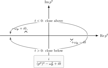
The Feynman prescription places the positive-energy pole below the real $p^0$ axis and the negative-energy pole above it. The factor $e^{-ip^0t}$ selects a clockwise lower closure for $t>0$ and a counterclockwise upper closure for $t<0$. The pole offsets and arcs are schematic boundary prescriptions, not the exact finite-$\epsilon$ roots derived above.

For $t>0$, the exponential $e^{-ip^0t}$ decays on the large semicircle in the lower half-plane, so the contour encloses the pole at $+\omega_{\mathbf p}-i0$. The residue gives

$$D_F(t,\mathbf p)={e^{-i\omega_{\mathbf p}t}\over2\omega_{\mathbf p}}.$$

For $t<0$, the contour closes in the upper half-plane and encloses the pole at $-\omega_{\mathbf p}+i0$, giving

$$D_F(t,\mathbf p)={e^{+i\omega_{\mathbf p}t}\over2\omega_{\mathbf p}}.$$

Therefore

$$D_F(t,\mathbf p)={1\over2\omega_{\mathbf p}}e^{-i\omega_{\mathbf p}|t|},$$

which is precisely the oscillator time-ordered correlator. Compare Schwartz 2014, § 6.2, pp. 75–77, translating the source’s $e^{+i\omega\tau}$ energy transform to the $e^{-ip^0t}$ transform used here; the sign of the contour closure follows from that exponential.

For a nonidentity Hermitian scalar primary of dimension $\Delta$ in a unitary conformal vacuum, the exact Euclidean two-point function has a positive normalization $C$:

$$G_E(x_E)={C\over |x_E|^{2\Delta}}.$$

The Wightman formulas below mean distributional limits. For example, the first is the limit of the smooth expression with $t-i\epsilon$ against test functions as $\epsilon\downarrow0$; it is not a pointwise function on the light cone. With the branch inherited from Euclidean signature, the boundary values are

$$\boxed{ W_+(t,\mathbf x)={C\over \left(\mathbf x^2-(t-i0)^2\right)^\Delta}, \qquad W_-(t,\mathbf x)={C\over \left(\mathbf x^2-(t+i0)^2\right)^\Delta}. }$$

Away from coincidence, the time-ordered correlator is

$$\boxed{ D_F(t,\mathbf x)={C\over\left(\mathbf x^2-t^2+i0\right)^\Delta}. }$$

This last formula is often the easiest one to remember, but it hides the more primitive statement: the $i0$ came from spectral analyticity and operator ordering.

The displayed time-ordered power is shorthand for a chosen local extension when its unrenormalized regulator limit fails at $x=0$. Different allowed extensions can differ by contact terms supported at coincidence. This freedom does not authorize arbitrary changes to the Wightman distributions: their original spectral boundary values must retain positivity and the spectrum condition. See Gillioz 2023, arXiv v3, § 3.4, pp. 27–29, and § 3.6, pp. 35–36 (PDF). His $W(x)=\langle\phi(0)\phi(x)\rangle$ is the reversed ordering, so the present $W_+(x)$ is his $W(-x)$; this translation fixes the sign of the imaginary displacement. The noncoincident ordering and causal-support comparison below remain fixed. A power law valid only at short distance is not an exact correlator at arbitrary timelike separation.

Vacuum commutator expectations as discontinuities

For a Hermitian scalar operator, the two Wightman functions determine the vacuum expectation value of the commutator:

$$C_O(t,\mathbf x) :=\langle\Omega|[O(t,\mathbf x),O(0)]|\Omega\rangle =W_+(t,\mathbf x)-W_-(t,\mathbf x).$$

This is not, in general, an identity between the operator-valued commutator and two c-number correlators. Microcausality is the separate, stronger operator statement that local bosonic operators commute at spacelike separation. A free-field commutator is exceptional: it is a c-number times the identity, so its vacuum expectation also gives the full commutator.

For a scalar primary two-point function, define

$$\rho=\mathbf x^2-t^2.$$

Then

$$W_+(t,\mathbf x)={C\over(\rho+i0\operatorname{sgn}t)^\Delta}, \qquad W_-(t,\mathbf x)={C\over(\rho-i0\operatorname{sgn}t)^\Delta}.$$

Thus the vacuum commutator expectation is the discontinuity across the branch cut of $\rho^{-\Delta}$:

$$\boxed{ C_O(t,\mathbf x) =C\left[ {1\over(\rho+i0\operatorname{sgn}t)^\Delta} -{1\over(\rho-i0\operatorname{sgn}t)^\Delta} \right]. }$$

If the separation is spacelike, then $\rho>0$. There is no branch cut, and the two boundary values agree. Therefore

$$C_O(t,\mathbf x)=0, \qquad \mathbf x^2>t^2.$$

This equality is the two-point reflection of causality. In a local theory, microcausality gives the operator identity $[O(t,\mathbf x),O(0)]=0$ throughout the same spacelike region (with a graded commutator for fermionic fields).

If the separation is timelike, then $\rho<0$. For non-integer $\Delta$, the two boundary values differ by a phase:

$$(\rho+i0)^{-\Delta}=e^{-i\pi\Delta}|\rho|^{-\Delta}, \qquad (\rho-i0)^{-\Delta}=e^{+i\pi\Delta}|\rho|^{-\Delta}.$$

Hence, pointwise in the timelike region away from the light cone,

$$C_O(t,\mathbf x) =-2iC\sin(\pi\Delta)\operatorname{sgn}(t) {\theta(t^2-\mathbf x^2)\over(t^2-\mathbf x^2)^\Delta}.$$

Globally, this expression denotes the distribution inherited from the original analytic Wightman boundary values, including any light-cone-supported terms. For $\Delta\ge1$, the displayed power times the step function is not by itself an ordinary locally integrable function at the light cone; a finite-part notation must represent that inherited boundary distribution rather than introduce an independent contact prescription.

The figure links the two sides of the negative-$\rho$ cut to a real spacetime section. Inspect where the cut is crossed and where the two boundary values agree; the shaded timelike region marks possible support, not a nonzero value for every conformal dimension.

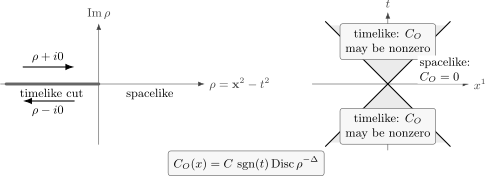
For a scalar conformal two-point function, the vacuum commutator expectation is the discontinuity across the negative-$\rho$ cut. For $t>0$, its upper bank gives $W_+$ and lower bank $W_-$; these assignments reverse for $t<0$. The spacelike values agree. Integer dimensions can leave light-cone-supported distributions even when the off-cone discontinuity vanishes. The geometry is schematic; operator microcausality is a separate, stronger statement.

All of these boundary values are distributions. Define the generalized principal value

$$\operatorname{Pf}\frac1{u^n} :=\frac{(-1)^{n-1}}{(n-1)!}\, \partial_u^{\,n-1}\operatorname{PV}\frac1u.$$

At a positive integer $n$, the terms supported exactly at the branch point are displayed by the one-variable identity

$$\boxed{ (u\pm i0)^{-n} =\operatorname{Pf}{1\over u^n} \mp i\pi {(-1)^{n-1}\over(n-1)!}\,\delta^{(n-1)}(u). }$$

Consequently,

$$(u+i0)^{-n}-(u-i0)^{-n} =-2\pi i\,{(-1)^{n-1}\over(n-1)!}\,\delta^{(n-1)}(u).$$

In particular, for the free massless scalar in four spacetime dimensions, $\Delta=1$ and the sine factor vanishes away from the light cone. The free commutator is nevertheless nonzero as a distribution; it is a c-number times the identity supported on the light cone:

$$[\phi(t,\mathbf x),\phi(0)] =-{i\over2\pi}\operatorname{sgn}(t)\delta(t^2-\mathbf x^2) \,\mathbf 1$$

for the standard four-dimensional normalization. This is the familiar sharp propagation of the massless free wave equation. For interacting conformal fields with anomalous dimensions, the vacuum commutator expectation generally has support throughout the timelike region.

Conformal covariance and Lorentzian distributions

For an implemented global map, the preceding lesson used the active primary-field rule

$$O(z,\bar z) \mapsto (f'(z))^h(\bar f'(\bar z))^{\bar h}O(f(z),\bar f(\bar z)).$$

Fix the Euclidean coordinate convention

$$x_E=(\tau,x), \qquad z=x+i\tau, \qquad \bar z=x-i\tau.$$

For a self-conjugate primary, the Euclidean two-point function on the plane is

$$\langle O(z,\bar z)O(0,0)\rangle ={C\over z^{2h}\bar z^{2\bar h}}.$$

For a charged or otherwise non-Hermitian primary, the operator at the origin is $O^\dagger$ instead. In either case, the complex powers require a specified branch.

This formula is single-valued only if the spin

$$s=h-\bar h$$

is compatible with the chosen spin structure. For the Ising Majorana fermion,

$$(h,\bar h)=\left({1\over2},0\right)$$

or

$$(h,\bar h)=\left(0,{1\over2}\right),$$

so the correlator is chiral:

$$\langle\psi(z)\psi(0)\rangle={1\over z}.$$

To pass to Lorentzian signature, introduce the light-cone coordinates

$$x^+=t+x, \qquad x^-=t-x.$$

For the ordering with the displayed operator first, continue from positive Euclidean time by setting $\tau=\epsilon+it$, with $\epsilon>0$. Then

$$z=-x^-+i\epsilon, \qquad \bar z=x^+-i\epsilon.$$

Thus the coordinate continuation of the Euclidean components, with their transported branches, is

$$\boxed{ \mathcal C_+(t,x) =\lim_{\epsilon\downarrow0} {C\over(-x^-+i\epsilon)^{2h}(x^+-i\epsilon)^{2\bar h}}. }$$

For a bosonic field, the other coordinate-side boundary follows from $\tau=-\epsilon+it$:

$$\boxed{ \mathcal C_-(t,x) =\lim_{\epsilon\downarrow0} {C\over(-x^--i\epsilon)^{2h}(x^++i\epsilon)^{2\bar h}}. }$$

For fermionic or semilocal fields, the coordinate-side prescriptions are the same, but the relative exchange or monodromy phase is fixed by the Euclidean graded-ordering and spin-structure conventions; it must not be inferred from the displayed bosonic formula alone.

For a scalar with the matched real normalization, these are the physical $W_\pm$ already derived. For spinful fields, $\mathcal C_\pm$ still need the continuation of the field components and their spin frames. For example, the unit holomorphic Euclidean pole at $t=x=0$ gives $1/(i\epsilon)=-i/\epsilon$. That cannot be the regulated coincident expectation of a Hermitian Lorentzian fermion, whose positive-energy spectral norm is real and nonnegative. The missing factors are consequential.

A normalized physical Majorana continuation

Let $\chi_R$ and $\chi_L$ be Hermitian real-time chiral fields, with

$$\{\chi_a(t,x),\chi_b(t,y)\}=\delta_{ab}\delta(x-y), \qquad a,b\in\{R,L\},$$

and action

$$S_L=\frac{i}{2}\int dt\,dx\, \big[\chi_R(\partial_t+\partial_x)\chi_R +\chi_L(\partial_t-\partial_x)\chi_L\big].$$

In Euclidean coordinates define $\partial=(\partial_x-i\partial_\tau)/2$ and $\bar\partial=(\partial_x+i\partial_\tau)/2$. The standard unit-pole Majorana normalization is

$$\begin{aligned} S_E&=\frac1{2\pi}\int d\tau\,dx\, \big(\psi\bar\partial\psi+\bar\psi\partial\bar\psi\big),\\ \langle\psi(z)\psi(0)\rangle_E&=\frac1z, \qquad \langle\bar\psi(\bar z)\bar\psi(0)\rangle_E=\frac1{\bar z}. \end{aligned}$$

The bar distinguishes the second Euclidean Grassmann field, rather than imposing an ordinary pointwise complex-conjugation condition. The action and unit pole are given in Di Francesco, Mathieu and Sénéchal 1997, § 5.3.2, pp. 129–131.

Wick rotation sends $\partial_t\to i\partial_\tau$ and $e^{iS_L}\to e^{-S_E}$. Before rescaling the fields, it produces the kinetic terms $-i\chi_R\bar\partial\chi_R$ and $+i\chi_L\partial\chi_L$ in $S_E$. Therefore one compatible continuation is

$$\chi_R^L\ \longrightarrow\ \frac{e^{i\pi/4}}{\sqrt{2\pi}}\psi_E, \qquad \chi_L^L\ \longrightarrow\ \frac{e^{-i\pi/4}}{\sqrt{2\pi}}\bar\psi_E.$$

Squaring each phase and substituting it into its kinetic term gives exactly the Euclidean action above. The same factors multiply the respective two-point functions. At finite $\epsilon>0$, the physical positive-frequency values are consequently

$$\begin{aligned} W_{R,\epsilon}^+(t,x) &=\frac{i}{2\pi(-x^-+i\epsilon)} =\int_0^\infty\frac{dk}{2\pi}\,e^{-ik(t-x)-\epsilon k},\\ W_{L,\epsilon}^+(t,x) &=\frac{-i}{2\pi(x^+-i\epsilon)} =\int_0^\infty\frac{dk}{2\pi}\,e^{-ik(t+x)-\epsilon k}. \end{aligned}$$

Both equal $1/(2\pi\epsilon)>0$ at regulated coincidence. Their limits define the physical Wightman distributions. For either chirality the reversed ordering is $W_a^+(-t,-x)$, without a time-ordering sign. Thus

$$\begin{aligned} W_R^+(t,x)+W_R^+(-t,-x)&=\delta(x^-),\\ W_L^+(t,x)+W_L^+(-t,-x)&=\delta(x^+), \end{aligned}$$

using $(u+i0)^{-1}-(u-i0)^{-1}=-2\pi i\delta(u)$. At equal time these recover the canonical anticommutators. In this free theory the anticommutators are c-numbers, so the check also determines the operator relation.

For complex fermions the fields paired by Lorentzian dagger continue to independent Euclidean Grassmann variables; their Wick phases are transported analytically, not obtained by simply complex-conjugating a phase after rotation. The state, branch, spin frame and field normalization all belong to a physical continuation. A change of coordinate names alone supplies only the denominators.

Example: recovering the equal-time canonical commutator

For the free scalar field, start from

$$[\phi(t,\mathbf x),\phi(0,\mathbf 0)] =\int {d^d\mathbf p\over(2\pi)^d}{1\over2\omega_{\mathbf p}} \left(e^{-i\omega_{\mathbf p}t+i\mathbf p\cdot\mathbf x}-e^{i\omega_{\mathbf p}t-i\mathbf p\cdot\mathbf x}\right).$$

Change $\mathbf p\mapsto-\mathbf p$ in the second term:

$$[\phi(t,\mathbf x),\phi(0,\mathbf 0)] =-i\int {d^d\mathbf p\over(2\pi)^d} {\sin(\omega_{\mathbf p}t)\over\omega_{\mathbf p}} e^{i\mathbf p\cdot\mathbf x}.$$

At equal time this vanishes:

$$[\phi(0,\mathbf x),\phi(0,\mathbf 0)]=0.$$

Differentiating with respect to $t$ gives

$$[\dot\phi(t,\mathbf x),\phi(0,\mathbf 0)] =-i\int {d^d\mathbf p\over(2\pi)^d} \cos(\omega_{\mathbf p}t)e^{i\mathbf p\cdot\mathbf x}.$$

At $t=0$,

$$[\dot\phi(0,\mathbf x),\phi(0,\mathbf 0)] =-i\delta^{(d)}(\mathbf x).$$

Equivalently,

$$[\phi(0,\mathbf x),\pi(0,\mathbf 0)] =i\delta^{(d)}(\mathbf x), \qquad \pi=\dot\phi.$$

Thus the same Wightman functions whose boundary values define the Feynman prescription also encode the canonical equal-time algebra.

Summary

A free field is a continuum of oscillators. Each oscillator gives two Wightman functions,

$$W_+(t)=\langle0|q(t)q(0)|0\rangle, \qquad W_-(t)=\langle0|q(0)q(t)|0\rangle,$$

and the field-theory correlators are momentum integrals of these elementary objects.

The spectrum condition defines $F_+$ in the lower half of the complex time plane and $F_-$ in the upper half-plane. The Wightman distributions $W_+$ and $W_-$ are their respective boundary values. The prescriptions $t-i0$ and $t+i0$ are therefore fixed by operator ordering.

The Feynman propagator glues the two Wightman functions with time-ordering step functions. In momentum space this is the pole prescription

$${ i\over p^2-m^2+i0}.$$

In conformal field theory, Euclidean power laws become Lorentzian distributions. With their boundary limits and branches understood, the scalar Wightman and Feynman forms are

$$W_+(t,\mathbf x)={C\over(\mathbf x^2-(t-i0)^2)^\Delta}, \qquad D_F(t,\mathbf x)={C\over(\mathbf x^2-t^2+i0)^\Delta}.$$

The difference of the two Wightman functions is the vacuum expectation value of the commutator. For a general interacting field this is not the full operator-valued commutator; local microcausality separately requires that operator to vanish at spacelike separation. Free-field commutators are the special c-number case.

Common pitfalls

Identifying time ordering with causal response. The raw Feynman correlator $D_F$ is time ordered. For a source-independent Hermitian operator and Hamiltonian perturbation $H_{\rm ext}(t)=-\int d^dx\,J(t,x)O(t,x)$, the causal response instead uses

$$\begin{aligned} \mathcal R(x)&=i\theta(t)\langle\Omega|[O(x),O(0)]|\Omega\rangle,\\ G_R(x)&=-i\theta(t)\langle\Omega|[O(x),O(0)]|\Omega\rangle =-\mathcal R(x). \end{aligned}$$

First-order Hamiltonian perturbation theory gives $\delta\langle O\rangle=\mathcal R*J$. This matches the response/retarded-correlator distinction in Lesson 7 and the Hamiltonian-source derivation. The source sign fixes the relation; renaming a kernel must not reverse the physical response.

Omitting the boundary prescription. A Lorentzian power with a singular or multivalued denominator needs its $i0$ and branch. A formal power is not a distribution until those data and any necessary extension are specified.

Choosing the side arbitrarily. For Wightman functions it is fixed by spectral positivity. Positive energies make the analytic function for $\langle\Omega|O(t)O(0)|\Omega\rangle$ converge below the real-time axis, so its boundary is approached from $t-i0$. A finite $\epsilon$ supplies exponential damping; $i0$ denotes the distributional limit after that regulator is removed.

Treating a time-ordered prescription as complete renormalization. The $i0$ fixes the side of the boundary value. Extending a sufficiently singular time-ordered correlator through coincidence can still require local counterterms. This does not license changes that violate the Wightman spectrum condition or positivity.

Exercises

Exercise 1: Oscillator time ordering

For $\omega>0$, let

$$q(t)={1\over\sqrt{2\omega}}(ae^{-i\omega t}+a^\dagger e^{i\omega t}).$$

Compute $\langle0|Tq(t)q(0)|0\rangle$ and show that it equals

$${1\over2\omega}e^{-i\omega|t|}.$$

Solution

For $t>0$,

$$\langle0|Tq(t)q(0)|0\rangle =\langle0|q(t)q(0)|0\rangle ={e^{-i\omega t}\over2\omega}.$$

For $t<0$,

$$\langle0|Tq(t)q(0)|0\rangle =\langle0|q(0)q(t)|0\rangle ={e^{i\omega t}\over2\omega}.$$

Since $t<0$ implies $|t|=-t$,

$$e^{i\omega t}=e^{-i\omega|t|}.$$

Thus in both cases

$$\langle0|Tq(t)q(0)|0\rangle ={1\over2\omega}e^{-i\omega|t|}.$$

Exercise 2: The Feynman energy contour

For $\omega>0$, use contour integration to prove

$$\int {dp^0\over2\pi}{i e^{-ip^0t}\over (p^0)^2-\omega^2+i0} ={1\over2\omega}e^{-i\omega|t|}.$$

Solution

Begin with a finite $\epsilon>0$ and define

$$\Omega_\epsilon=\sqrt{\omega^2-i\epsilon}, \qquad \operatorname{Re}\Omega_\epsilon>0, \quad \operatorname{Im}\Omega_\epsilon<0.$$

The exact poles are $p^0=\Omega_\epsilon$ in the lower half-plane and $p^0=-\Omega_\epsilon$ in the upper half-plane. For $t>0$, close clockwise below. The residue is

$$\operatorname{Res}_{p^0=\Omega_\epsilon} {i e^{-ip^0t}\over (p^0-\Omega_\epsilon)(p^0+\Omega_\epsilon)} ={i e^{-i\Omega_\epsilon t}\over2\Omega_\epsilon}.$$

The clockwise contour therefore gives

$$I_\epsilon(t>0) ={e^{-i\Omega_\epsilon t}\over2\Omega_\epsilon}.$$

For $t<0$, close counterclockwise above. The residue at $p^0=-\Omega_\epsilon$ is

$$\operatorname{Res}_{p^0=-\Omega_\epsilon} {i e^{-ip^0t}\over (p^0-\Omega_\epsilon)(p^0+\Omega_\epsilon)} =-{i e^{i\Omega_\epsilon t}\over2\Omega_\epsilon},$$

so

$$I_\epsilon(t<0) ={e^{i\Omega_\epsilon t}\over2\Omega_\epsilon}.$$

Taking $\epsilon\downarrow0$ sends $\Omega_\epsilon\to\omega$ and gives $I(t)=e^{-i\omega|t|}/(2\omega)$ in both cases.

Exercise 3: Equality at spacelike separation

Let

$$F_\Delta(t,\mathbf x)={1\over\left(\mathbf x^2-(t-i0)^2\right)^\Delta}.$$

Show that, for spacelike separation $\mathbf x^2>t^2$, the two Wightman boundary values

$${1\over(\mathbf x^2-(t-i0)^2)^\Delta} \quad\text{and}\quad {1\over(\mathbf x^2-(t+i0)^2)^\Delta}$$

are equal.

Solution

Write

$$\rho=\mathbf x^2-t^2.$$

The two denominators are

$$\mathbf x^2-(t-i0)^2=\rho+i0\operatorname{sgn}t,$$

and

$$\mathbf x^2-(t+i0)^2=\rho-i0\operatorname{sgn}t.$$

For spacelike separation, $\rho>0$. The function $\rho^{-\Delta}$ has no branch cut on the positive real axis, so approaching from above or below gives the same boundary value:

$$(\rho+i0)^{-\Delta}=(\rho-i0)^{-\Delta}=\rho^{-\Delta}.$$

Thus their discontinuity vanishes for spacelike separation. When these are two-point functions, this is the vanishing vacuum commutator expectation; microcausality is the corresponding operator statement.

Exercise 4: The timelike branch-cut discontinuity

For non-integer $\Delta$, compute the discontinuity

$$(\rho+i0)^{-\Delta}-(\rho-i0)^{-\Delta}$$

for $\rho<0$, using the principal branch of the logarithm.

Solution

For $\rho<0$, write $\rho=-|\rho|$. On the principal branch,

$$\rho+i0=|\rho|e^{i\pi}, \qquad \rho-i0=|\rho|e^{-i\pi}.$$

Therefore

$$(\rho+i0)^{-\Delta}=|\rho|^{-\Delta}e^{-i\pi\Delta},$$

and

$$(\rho-i0)^{-\Delta}=|\rho|^{-\Delta}e^{+i\pi\Delta}.$$

Their difference is

$$(\rho+i0)^{-\Delta}-(\rho-i0)^{-\Delta} =|\rho|^{-\Delta}\left(e^{-i\pi\Delta}-e^{i\pi\Delta}\right) =-2i\sin(\pi\Delta)|\rho|^{-\Delta}.$$

If the boundary values are instead $\rho\pm i0\operatorname{sgn}t$, this result is multiplied by $\operatorname{sgn}t$.

Exercise 5: Spectral analyticity

Let the positive spectral measure have at most polynomial cumulative growth, $\mu([0,E])\le A(1+E)^N$, as in the half-plane argument above. Starting from the corresponding spectral sum

$$F_+(z)=\sum_n c_n e^{-iE_nz}, \qquad c_n\ge0, \qquad E_n\ge0,$$

explain why $F_+(z)$ is analytic for $\operatorname{Im}z<0$ but not generally for $\operatorname{Im}z>0$, and identify the real-time Wightman distribution.

Solution

Let $z=t_R+i t_I$. Then

$$e^{-iE_n z}=e^{-iE_n t_R}e^{E_n t_I}.$$

If $t_I<0$, the factor $e^{E_n t_I}$ damps high-energy contributions. This makes the spectral sum, or its continuum version, well behaved in the lower half-plane under the usual assumptions on the growth of spectral weights.

If $t_I>0$, the same factor grows exponentially with $E_n$. There is no reason for the spectral sum to converge there. The reversed ordering has phases $e^{+iE_n z}$ and is analytic in the upper half-plane instead. The real-time Wightman distribution is the lower-half-plane boundary value

$$W_+(t)=\lim_{\epsilon\downarrow0}F_+(t-i\epsilon)$$

in the sense of distributions.

References

• Di Francesco, Philippe, Pierre Mathieu, and David Sénéchal. Conformal Field Theory. Graduate Texts in Contemporary Physics. Springer, 1997. DOI.
• Gillioz, Marc. Conformal Field Theory for Particle Physicists: From QFT Axioms to the Modern Conformal Bootstrap. SpringerBriefs in Physics. Springer, 2023. DOI. Open PDF, arXiv:2207.09474v3, 3 May 2023. Locators above use the preprint’s printed page labels.
• Schwartz, Matthew D. Quantum Field Theory and the Standard Model. Cambridge University Press, 2014. DOI.

Further reading

This lesson preserves the oscillator-to-CFT lecture sequence. For a broader structural account of ordered vacuum correlators, see Wightman functions and spectral support; for vacuum selection, causal prescriptions, and Wick rotation, see Lorentzian boundary conditions and the iε prescription.