Stress Tensors, Goldstone Modes, and QED Ward Identities

A Ward identity specifies both a conservation law away from insertions and the contact terms that implement a symmetry on those insertions. This lesson applies that distinction to a broken global symmetry, the stress tensor and the proper QED vertex. A nonzero order-parameter contact forces a singular longitudinal current correlator; the additional spectral hypotheses give its Goldstone interpretation. A local translation instead differentiates the inserted operators.

The stress-tensor derivation is Euclidean and keeps the sign of metric variation explicit. The QED vertex is defined first in Lorentzian Feynman conventions; its photon self-energy is then continued to nonzero Euclidean momentum. The final two-dimensional calculation relates the metric tensor to the residue-normalized holomorphic field $T(z)$, including its factor of $2\pi$.

Required background. Lesson 18 supplies the localized-symmetry derivation of current Ward identities and their contact terms. Helpful background. Lessons 13–16 develop scale and conformal transformations; only their basic geometric action is used here.

Goldstone pole from a Ward identity

Let $J_\mu$ be the current of a nonanomalous continuous global symmetry. Factor its local infinitesimal parameter out of the transformation:

$$\delta_\alpha\Phi=\alpha\,\Delta\Phi, \qquad \delta_\alpha S_E=\int d^d x\,J_\mu\partial_\mu\alpha.$$

Here $\Delta\Phi$ is the generator’s action, not a variation still containing $\alpha$. The Euclidean change of variables from Lesson 18 gives

$$\partial_\mu\langle J_\mu(x)\Phi(0)\rangle =-\delta^{(d)}(x)\langle\Delta\Phi(0)\rangle.$$

Select an infinite-volume vacuum by taking the volume limit before removing a symmetry-breaking source. A broken phase has a local order parameter for which

$$B\equiv\langle\Delta\Phi\rangle\ne0.$$

Fourier transforming the Ward identity gives

$$q_\mu C_\mu(q)=-iB, \qquad C_\mu(q)=\int d^d x\,e^{iq\cdot x}\langle J_\mu(x)\Phi(0)\rangle.$$

A derivative transforms to $-iq_\mu$, which fixes the displayed factor of $i$. At nonzero Euclidean momentum, the exact longitudinal projection is

$$C_\mu^{\parallel}(q)=-iB\,{q_\mu\over q_E^2}, \qquad q_E^2=\sum_\mu q_\mu^2>0.$$

A correlator bounded near the origin cannot satisfy this identity. Rotational invariance of a scalar-order-parameter vacuum leaves no additional vector direction; more generally the Ward equation leaves transverse terms undetermined. The pole and regular control in Lesson 18 show why a regular term cannot replace this singularity.

The physical Goldstone conclusion additionally requires a translation- and Lorentz-invariant vacuum, a local conserved current, a positive physical energy spectrum, and the regulated local charge-commutator limit that implements the symmetry. Under these hypotheses the current–order-parameter spectral representation has a massless contribution. When described by a one-particle Goldstone state, its current matrix element can be normalized as

$$\langle0|J^L_\mu(0)|\pi(q)\rangle=iFq_\mu,$$

where $J^L$ is the corresponding Lorentzian current, with nonzero $F$ and a suitable state phase. Inserting the massless state supplies the pole. This spectral step is developed in Weinberg 1995, Volume II, § 19.2, pp. 169–172. It does not require an unsmeared global charge to act as a finite-norm operator on the broken vacuum.

In relativistic $1+1$ dimensions, the continuously broken vacuum just described is excluded under Coleman’s local, positive-spectrum assumptions; this is not a prohibition of every massless state (Coleman 1973, pp. 259–264, Open PDF). A gauge redundancy also does not meet the physical global-symmetry premises. In a Higgs description, a would-be Goldstone field can supply the longitudinal massive-vector polarization without an additional physical massless particle.

Stress tensor as the current for translations

Consider first scalar fields and a first-derivative Euclidean density $\mathcal L_E(\phi^a,\partial_\mu\phi^a)$ with no explicit coordinate dependence. At fixed coordinates and metric, localize an active translation as

$$\delta_\xi\phi^a(x)=\xi^\nu(x)\partial_\nu\phi^a(x),$$

with smooth compactly supported $\xi$. Differentiating the density gives a total derivative plus the Noether term:

$$\delta_\xi\mathcal L_E =\partial_\mu(\xi^\mu\mathcal L_E) +T^{\mathrm{can}}_{\mu\nu}\partial_\mu\xi_\nu,$$

where

$$T_{\mu\nu}^{\mathrm{can}} ={\partial\mathcal L_E\over\partial(\partial_\mu\phi^a)}\partial_\nu\phi^a -\delta_{\mu\nu}\mathcal L_E.$$

Thus $\delta_\xi S_E=\int T^{\mathrm{can}}_{\mu\nu}\partial_\mu\xi_\nu$. On the equations of motion, the same compactly supported field variation has zero action variation, and integration by parts gives

$$\partial_\mu T^{\mathrm{can}}_{\mu\nu}=0.$$

An arbitrary local translation is not itself a global symmetry of a fixed background. Its variation defines the current; the field equations give conservation. Off shell, with $E_a=\delta S_E/\delta\phi^a$, the same calculation gives

$$\partial_\mu T^{\mathrm{can}}_{\mu\nu}=-E_a\partial_\nu\phi^a.$$

One may add an identically conserved improvement,

$$T_{\mu\nu}\mapsto T_{\mu\nu}+\partial_\rho B_{\rho\mu\nu}, \qquad B_{\rho\mu\nu}=-B_{\mu\rho\nu},$$

without changing the corresponding charge when the surface contribution vanishes. For fields with spin, the local transformation also acts on their indices. The following metric construction gives a symmetric tensor and makes the Euclidean sign explicit.

Metric variation and diffeomorphism Ward identities

Vary the covariant background metric while holding the matter field fixed, and define $T^{\mu\nu}$ by

$$\delta_g S_E={1\over2}\int d^d x\sqrt g\,T^{\mu\nu}\delta g_{\mu\nu}.$$

This sign matters. For a minimally coupled real scalar,

$$S_E=\int d^d x\sqrt g\left[\frac12g^{\mu\nu} \partial_\mu\phi\partial_\nu\phi+V(\phi)\right], \qquad T^{\mu\nu}=g^{\mu\nu}\mathcal L_E-\nabla^\mu\phi\nabla^\nu\phi.$$

The identities $\delta\sqrt g=\frac12\sqrt g\,g^{\mu\nu}\delta g_{\mu\nu}$ and $\delta g^{\alpha\beta}=-g^{\alpha\mu}g^{\beta\nu}\delta g_{\mu\nu}$ give this result directly. In flat space, this metric tensor is $-T^{\mathrm{can}}$ for the scalar. The sign is additional to any improvement freedom. Di Francesco et al. use the opposite metric definition, so their tensor is $-T$ here (Di Francesco, Mathieu and Sénéchal 1997, § 2.5.2, pp. 49–50).

A simultaneous pullback of the metric and scalar has

$$\delta g_{\mu\nu}=\nabla_\mu\xi_\nu+\nabla_\nu\xi_\mu.$$

The matter variation is $\delta_\xi\phi=\xi^\nu\nabla_\nu\phi$. Write $E_\phi=(\sqrt g)^{-1}\delta S_E/\delta\phi$. The full diffeomorphism variation, rather than the metric variation alone, is

$$0=\delta_{g,\phi}S_E =\int d^d x\sqrt g\left( T^{\mu\nu}\nabla_\mu\xi_\nu+E_\phi\xi^\nu\nabla_\nu\phi\right).$$

Compact support removes the boundary term. Since $\xi$ is arbitrary,

$$\nabla_\mu T^{\mu\nu}=E_\phi\nabla^\nu\phi.$$

On shell this becomes

$$\boxed{\nabla_\mu T^{\mu\nu}=0.}$$

The scalar example also clarifies continuation to physical momentum. Let $\Theta^L_{\mu\nu}=\partial_\mu\phi\partial_\nu\phi-\eta_{\mu\nu}\mathcal L_L$. Under $t=-i\tau$, the continued components obey $\Theta^L_{00}\mapsto T_{\tau\tau}$ and $\Theta^L_{0i}\mapsto-iT_{\tau i}$, since $\partial_\tau\phi=-i\partial_t\phi$. The physical charges are $P^\nu=\int d^{d-1}\mathbf x\,\Theta_L^{0\nu}$ (Schwartz 2014, § 3.3.1, pp. 34–36). Integrating the Euclidean canonical tensor as though it were a Lorentzian energy density would miss these signs and factors.

The figure illustrates the pullback with one exact map on a flat patch. Both grid families use $F_a(x,y)=(x+ay^2,y)$, whose Jacobian and metric are

$$DF_a=\begin{pmatrix}1&2ay\\0&1\end{pmatrix}, \qquad F_a^*\delta=\begin{pmatrix}1&2ay\\2ay&1+4a^2y^2\end{pmatrix}.$$

Thus $\det DF_a=1$ and the first-order off-diagonal variation is $2ay$, exactly the symmetric gradient of $\xi=(ay^2,0)$. This coordinate deformation introduces no curvature.

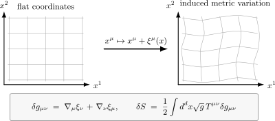
Both grid families are images of $F_a(x,y)=(x+ay^2,y)$ with $a=0.18$ and $-1\le x,y\le1$ in dimensionless coordinates. The two grids have the same plotting scale. The exact Jacobian gives the finite pullback metric; the displayed $\delta g^{(1)}$ retains only its term linear in $a$. Conservation requires the simultaneous matter variation, not just the pictured metric change.

At fixed flat metric, the active scalar variation instead gives $\delta_\xi S_E=-\int T_{\mu\nu}\partial_\mu\xi_\nu=\int\xi_\nu\partial_\mu T_{\mu\nu}$. For a measure and renormalization prescription preserving diffeomorphism symmetry, insert this into $0=\langle\delta\mathcal O\rangle-\langle\mathcal O\delta S_E\rangle$. If the inserted scalar operators transform as $\delta O_i=\xi^\nu\partial_\nu O_i$, the result is

$$\boxed{ \partial_\mu\left\langle T_{\mu\nu}(x)\prod_i O_i(x_i)\right\rangle =+\sum_i\delta^{(d)}(x-x_i){\partial\over\partial x_i^\nu} \left\langle\prod_i O_i(x_i)\right\rangle. }$$

The positive contact follows from the chosen metric definition. The canonical Euclidean tensor has the opposite contact. Operators carrying indices or density weight acquire additional derivative-of-parameter contacts; renormalized composite operators can have mixing contacts. A gravitational anomaly or a boundary also requires the corresponding additional terms.

Rotations, dilatations, and conformal transformations

Special choices of $\xi_\mu(x)$ turn the stress-tensor Ward identity into familiar spacetime symmetries.

For rotations,

$$\xi_\nu=\omega_{\nu\rho}x_\rho, \qquad \omega_{\nu\rho}=-\omega_{\rho\nu},$$

so

$$\partial_\mu\xi_\nu=\omega_{\nu\mu}.$$

Only an antisymmetric tensor component could contribute to this contraction. The metric tensor is already symmetric by definition. For the canonical tensor, local rotation invariance and a local spin current allow the Belinfante improvement to a symmetric tensor,

$$T_{\mu\nu}=T_{\nu\mu}.$$

For fields with spin, this improvement is the Belinfante construction. The angular-momentum current is schematically

$$M_{\lambda\mu\nu}=x_\mu T_{\lambda\nu}^{\mathrm{can}} -x_\nu T_{\lambda\mu}^{\mathrm{can}} +S_{\lambda\mu\nu},$$

where $S_{\lambda\mu\nu}$ is the spin current. Conservation of $M_{\lambda\mu\nu}$ says that the antisymmetric part of $T^{\mathrm{can}}$ is a total derivative, which can be absorbed into an improvement.

For a dilation,

$$\xi_\nu=\lambda x_\nu, \qquad \partial_\mu\xi_\nu=\lambda\delta_{\mu\nu}.$$

The metric-only variation becomes

$$\delta_g S_E=\lambda\int d^d x\,T^\mu{}_{\mu}.$$

The field scaling transformation must also be included in a dilation Ward identity. For a local scale current, its on-shell conservation gives a trace of the form

$$T^\mu{}_{\mu}=\partial_\mu V^\mu$$

for a virial current $V^\mu$, whose sign is defined by this equation. If an allowed local improvement removes this divergence, one can choose

$$\boxed{T^\mu{}_{\mu}=0.}$$

These statements have different hypotheses:

Transformation	Local tensor statement	Conditions
Translation	$\partial_\mu T_{\mu\nu}=0$ away from insertions	Field equations, or the nonanomalous correlator Ward identity with its insertion contacts
Rotation	$T_{\mu\nu}=T_{\nu\mu}$	Metric definition, or a local Belinfante improvement including the spin current
Dilation and conformal transformation	$T^\mu{}_{\mu}=\partial_\mu V^\mu$, then possibly $T^\mu{}_{\mu}=0$	A local scale current, then a removable virial term; quantum anomalies and boundary terms must be treated separately

A conformal transformation is generated by a vector field satisfying the conformal Killing equation

$$\partial_\mu\xi_\nu+\partial_\nu\xi_\mu ={2\over d}(\partial\cdot\xi)\delta_{\mu\nu}.$$

If $T_{\mu\nu}$ is symmetric and traceless, then

$$T_{\mu\nu}\partial_\mu\xi_\nu ={1\over2}T_{\mu\nu}(\partial_\mu\xi_\nu+\partial_\nu\xi_\mu) ={1\over d}(\partial\cdot\xi)T^\mu{}_{\mu}=0.$$

Thus a symmetric, conserved, traceless stress tensor gives the local conformal currents, with the appropriate insertion transformations in their Ward identities. For the underlying canonical tensor and rotation-current construction, see Di Francesco, Mathieu and Sénéchal 1997, § 2.5, pp. 45–46.

For $d>2$, the conformal Killing equation has finitely many independent solutions: translations, rotations, dilatations, and special conformal transformations. The infinitesimal special conformal transformation is

$$\xi^\mu(x)=2(b\cdot x)x^\mu-b^\mu x^2.$$

Equivalently, the finite map can be written as inversion, translation, inversion:

$${x'^{\mu}\over x'^2}={x^\mu\over x^2}-b^\mu,$$

where the minus sign in the translation parameter is fixed by the convention above.

Scale invariance versus conformal invariance

The implication from scale invariance to conformal invariance is not a purely algebraic identity. The safe local criterion is the existence of a conserved symmetric stress tensor whose trace can be improved to zero. Many unitary relativistic critical theories of interest satisfy this criterion, but it should not be used without checking its assumptions.

QED Ward–Takahashi identity

Use Lorentzian QED with interaction $\mathcal L_{\rm int}=-e\bar\psi\gamma^\mu\psi A_\mu$, $e>0$. Relative to the site’s signed charge convention this is $q_{\rm site}=-e$: $\psi\mapsto e^{-ie\alpha}\psi$ and $A_\mu\mapsto A_\mu+\partial_\mu\alpha$. Define the matrix-valued stripped fermion propagator $G$ by

$$S_F(p)=iG(p), \qquad G^{-1}(p)=p\!\!\!/ -m-\Sigma(p), \qquad p\!\!\!/\equiv\gamma^\mu p_\mu.$$

The usual Feynman boundary prescription is understood; matrix inversion is used at nonsingular off-shell momenta. Define the proper photon vertex by its Feynman insertion $-i\Gamma_\mu(p+q,p)$, so its tree value is $e\gamma_\mu$. It is the three-point derivative of the one-particle-irreducible effective action, with fermion momentum $p$ entering, $p+q$ leaving, and photon momentum $q$ entering. This fixes the overall charge and $i$ factors; $G$ is not the raw time-ordered correlator $S_F$.

To derive the identity, let $K(x-y)$ be the quadratic fermion kernel of the effective action and $-V_\mu(x,y;z)$ its coefficient of $\bar\psi(x)\psi(y)A^\mu(z)$. Remove the known quadratic gauge-fixing term before applying its gauge identity. Under the transformations just stated, the terms bilinear in the fermions give

$$\partial_z^\mu V_\mu(x,y;z) =-ie\,[\delta^{(d)}(z-x)-\delta^{(d)}(z-y)]K(x-y).$$

This follows directly: the fermion variation of the quadratic term is $ie[\alpha(x)-\alpha(y)]\bar\psi(x)K(x-y)\psi(y)$, while integration by parts in the photon variation supplies $\partial_z^\mu V_\mu$. The identity assumes a regulator and counterterms preserving the vector gauge symmetry. The distinction between the connected generator and the vertex effective action, including the separated gauge-fixing term, is explicit in Zinn-Justin 2021, § 21.9, pp. 526–527.

Fourier transform the three-point kernel with $e^{+ip'\cdot x-ip\cdot y-iq\cdot z}$ and remove the common translation delta function, with $p'=p+q$. The transformed kernels are $K(p)=G^{-1}(p)$ and $V_\mu(p',p)=\Gamma_\mu(p',p)$. The two contacts give $K(p)$ and $K(p')$, respectively; the derivative gives $+iq^\mu$. Thus

$$\boxed{ q^\mu\Gamma_\mu(p+q,p) =e\left[G^{-1}(p+q)-G^{-1}(p)\right]. }$$

This is the Ward–Takahashi identity. Its tree check is $q^\mu e\gamma_\mu=e[(p+q)\!\!\!/-m-(p\!\!\!/-m)]$. In Schwartz’s convention the charge is outside the vertex, so the present $\Gamma$ equals $e\Gamma_{\rm Schwartz}$ (Schwartz 2014, § 19.5.1, p. 352, Eqs. 19.74–19.80).

A full connected insertion of $j_\mu=e\bar\psi\gamma_\mu\psi$, amputated only in its fermion legs, need not be this proper photon vertex: dynamical photons allow additional photon-reducible transverse contributions. At tree level its two ordered fermion contractions give $S_F(p+q)e\gamma_\mu S_F(p)$, consistently with the normalization above. The all-orders proper identity follows from the effective action, rather than identifying those two different three-point objects.

If $G^{-1}$ is differentiable at the chosen off-shell $p$, then

$$G^{-1}(p+q)=G^{-1}(p)+q^\nu{\partial G^{-1}(p)\over\partial p^\nu}+o(|q|).$$

If the vertex also has a direction-independent continuous limit as $q\to0$, take $q=\epsilon n$ for arbitrary fixed $n$, divide the Ward identity by $\epsilon$, and obtain

$$\boxed{ \Gamma_\mu(p,p)=e{\partial G^{-1}(p)\over\partial p^\mu}. }$$

This soft limit requires the stated regularity; an infrared or on-shell singularity can obstruct it. In a compatible perturbative renormalization prescription, the Ward identity yields $Z_1=Z_2$. Charge renormalization also involves photon normalization, so this equality alone does not say that the physical charge is unchanged.

Transverse photon self-energy

The second photon derivative of the same gauge identity makes the self-energy transverse. Continue it to a parity-even, rotation-invariant Euclidean vacuum and restrict to $q_E^2>0$:

$$\boxed{q_\mu\Pi_{\mu\nu}(q)=0.}$$

The symmetric tensor can contain only $\delta_{\mu\nu}$ and $q_\mu q_\nu$. Contracting their general linear combination with $q_\mu$ gives

$$\Pi_{\mu\nu}(q)=\left(q_E^2\delta_{\mu\nu}-q_\mu q_\nu\right)\Pi(q_E^2) =q_E^2\Pi(q_E^2)(P_T)_{\mu\nu}, \qquad (P_T)_{\mu\nu}=\delta_{\mu\nu}-{q_\mu q_\nu\over q_E^2}.$$

A local Proca contribution to the self-energy would be proportional to $m_\gamma^2\delta_{\mu\nu}$. Contracting with $q_\mu$ gives $m_\gamma^2q_\nu$, so such a term violates the Ward identity unless $m_\gamma^2=0$.

This statement concerns the self-energy, not the entire gauge-fixed inverse propagator, whose longitudinal gauge-fixing part is prescribed separately. Transversality alone does not forbid every gauge-invariant mass gap. For example, $\Pi(q_E^2)=m_\gamma^2/q_E^2$ gives $\Pi_{\mu\nu}=m_\gamma^2(P_T)_{\mu\nu}$. It is transverse at every nonzero Euclidean momentum, but its limit at zero depends on direction. Such a nonanalytic structure is allowed by the identity; whether it occurs requires a dynamical calculation, as in the Schwinger model.

Inspect the projection in the figure: the parallel component is removed and the perpendicular one survives. The lower comparison tests the two mass tensors on $q$ itself.

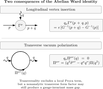
The Euclidean projector acts on $q=(1,0)$ and $v=(1.4,1)$ in an illustrative two-dimensional component plane, giving $P_Tv=(0,1)$. For $m_\gamma^2>0$, the local Proca self-energy $m_\gamma^2I$ is not transverse; $m_\gamma^2P_T$ is transverse but nonanalytic at $q=0$. This exact linear-algebra comparison permits a tensor structure without asserting its dynamical generation.

Notice what the Ward–Takahashi identity does not say. It fixes the longitudinal part of the vertex. It does not determine all transverse structures. Those contain genuine dynamics, such as anomalous magnetic moments and form factors.

Two-dimensional stress tensor and holomorphy

In two Euclidean dimensions define

$$z=x^1+i x^2, \qquad \bar z=x^1-i x^2,$$

so

$$ds^2=(dx^1)^2+(dx^2)^2=dz\,d\bar z.$$

Write $T^{\rm metric}_{ab}$ for the tensor defined by metric variation above. Its complex components obey

$$T^{\rm metric}_{zz}={1\over4} \left(T^{\rm metric}_{11}-T^{\rm metric}_{22}-2iT^{\rm metric}_{12}\right),$$

and

$$T^{\rm metric}_{\bar z\bar z}={1\over4} \left(T^{\rm metric}_{11}-T^{\rm metric}_{22}+2iT^{\rm metric}_{12}\right).$$

The mixed component is proportional to the trace:

$$T^{\rm metric}_{z\bar z}={1\over4} \left(T^{\rm metric}_{11}+T^{\rm metric}_{22}\right).$$

For a traceless improved tensor in a flat conformal vacuum,

$$T^{\rm metric}_{z\bar z}=0.$$

Stress-tensor conservation then splits into

$$\bar\partial T^{\rm metric}_{zz}=0, \qquad \partial T^{\rm metric}_{\bar z\bar z}=0$$

away from insertions. With $d^2z\equiv dx^1dx^2$ and the plus metric-variation convention in this page, the standard residue-normalized CFT fields are

$$T(z)=2\pi T^{\rm metric}_{zz}(z), \qquad \overline T(\bar z)=2\pi T^{\rm metric}_{\bar z\bar z}(\bar z).$$

The three components have distinct roles:

Component	CFT interpretation	Flat-space condition away from insertions
$T^{\rm metric}_{z\bar z}$	One quarter of the Cartesian trace	Vanishes for the traceless improved tensor
$T^{\rm metric}_{zz}$	$T(z)=2\pi T^{\rm metric}_{zz}$	$\bar\partial T=0$
$T^{\rm metric}_{\bar z\bar z}$	$\bar T(\bar z)=2\pi T^{\rm metric}_{\bar z\bar z}$	$\partial\bar T=0$

The factor is fixed by the contour normalization $Q_\epsilon=(2\pi i)^{-1}\oint dz\,\epsilon(z)T(z)$ and the standard primary-field transformation. In Di Francesco et al.’s opposite metric convention the corresponding formula is $T_{\rm CFT}=-2\pi T_{{\rm source},zz}$, giving the plus sign here (Di Francesco, Mathieu and Sénéchal 1997, § 5.2, pp. 119–120).

A free-scalar check fixes both the sign and magnitude. For $S_E=\frac{g_0}{2}\int d^2x\,(\partial_a\phi)^2$, $g_0>0$, the local covariance is

$$\langle\phi(z)\phi(w)\rangle =-\frac{1}{4\pi g_0}\log\big(\mu^2|z-w|^2\big), \qquad T^{\rm metric}_{zz}=-g_0:(\partial\phi)^2:.$$

The arbitrary infrared scale drops out of derivative correlators; this is a local derivative-sector check, not an assertion of a normalizable scalar zero-mode vacuum. Differentiating the logarithm and making the two single contractions in $T(z)\partial\phi(w)$ gives

$$T(z)\partial\phi(w) \sim\frac{\partial\phi(w)}{(z-w)^2} +\frac{\partial^2\phi(w)}{z-w}, \qquad T=-2\pi g_0:(\partial\phi)^2:.$$

The double-pole coefficient is one, as required for the weight-one field $\partial\phi$. A missing $2\pi$ or the opposite metric sign fails this check. Local conformal transformations

$$z\mapsto f(z), \qquad \bar z\mapsto \bar f(\bar z)$$

are therefore generated by contour integrals of $T(z)$ and $\overline T(\bar z)$ on their domains of definition. Their local contour action need not extend to a globally defined conformal map of the full surface.

Common pitfalls

Conservation without symmetry breaking. A conserved global current forces the singularity discussed here only when $\langle\Delta\Phi\rangle\ne0$. Its physical Goldstone interpretation also uses the declared vacuum and spectrum assumptions.

Metric sign versus improvement. With this page’s plus covariant-metric variation, the minimally coupled scalar has $T^{\rm metric}=-T^{\rm can}$ in Euclidean signature. This overall sign is not an improvement; compare charges only after specifying the same signature and continuation.

Flat tracelessness versus curved trace. Tracelessness is a local operator statement modulo contact terms and allowed improvements. Curved-background trace anomalies can remain in a theory whose flat-space improved tensor is traceless.

Current insertion versus proper vertex. The Ward–Takahashi identity fixes the longitudinal part of the proper QED vertex. It neither determines transverse form factors nor identifies a full current insertion with a one-particle-irreducible photon vertex.

Transverse versus massless. A local Proca self-energy $m_\gamma^2\delta_{\mu\nu}$ fails the transverse test. A nonanalytic transverse structure can instead contribute to a physical mass scale; transversality alone establishes neither its presence nor its absence.

Exercises

Exercise 1: Diffeomorphism Ward identity

Starting from

$$\delta_g S_E={1\over2}\int d^d x\sqrt g\,T^{\mu\nu}\delta g_{\mu\nu}$$

and

$$\delta g_{\mu\nu}=\nabla_\mu\xi_\nu+\nabla_\nu\xi_\mu,$$

include the scalar variation $\delta\phi=\xi^\nu\nabla_\nu\phi$ and derive the off-shell identity. State when it reduces to $\nabla_\mu T^{\mu\nu}=0$.

Solution

Substitute the metric variation:

$$\delta_g S_E={1\over2}\int d^d x\sqrt g\,T^{\mu\nu} (\nabla_\mu\xi_\nu+\nabla_\nu\xi_\mu).$$

Because $T^{\mu\nu}$ is symmetric in the metric definition,

$$\delta_g S_E=\int d^d x\sqrt g\,T^{\mu\nu}\nabla_\mu\xi_\nu.$$

Integrating by parts gives

$$\delta_g S_E=-\int d^d x\sqrt g\,\xi_\nu\nabla_\mu T^{\mu\nu}$$

for compactly supported $\xi$. The accompanying matter variation is $\delta_\phi S_E=\int d^dx\sqrt g\,E_\phi\xi_\nu\nabla^\nu\phi$. Invariance of the sum gives

$$0=\int d^dx\sqrt g\,\xi_\nu \left(-\nabla_\mu T^{\mu\nu}+E_\phi\nabla^\nu\phi\right).$$

Hence $\nabla_\mu T^{\mu\nu}=E_\phi\nabla^\nu\phi$. On the matter equations of motion $E_\phi=0$,

$$\nabla_\mu T^{\mu\nu}=0.$$

Exercise 2: Belinfante symmetry from rotations

For the canonical Euclidean tensor, let

$$\delta_\xi S_E=\int d^d x\,T^{\rm can}_{\mu\nu}\partial_\mu\xi_\nu.$$

Show that the orbital part of a rotation $\xi_\nu=\omega_{\nu\rho}x_\rho$, with $\omega_{\nu\rho}=-\omega_{\rho\nu}$, couples only to its antisymmetric part. Explain what additional information is needed for a Belinfante improvement when fields carry spin.

Solution

In this solution abbreviate $T^{\rm can}_{\mu\nu}$ as $T_{\mu\nu}$. For the orbital rotation,

$$\partial_\mu\xi_\nu=\omega_{\nu\mu}.$$

Thus

$$\delta S=\int d^d x\,T_{\mu\nu}\omega_{\nu\mu}.$$

Decompose

$$T_{\mu\nu}=T_{(\mu\nu)}+T_{[\mu\nu]},$$

where the first term is symmetric and the second is antisymmetric. Since $\omega_{\nu\mu}$ is antisymmetric,

$$T_{(\mu\nu)}\omega_{\nu\mu}=0.$$

Therefore

$$\delta S=\int d^d x\,T_{[\mu\nu]}\omega_{\nu\mu}.$$

This contraction by itself does not construct an improvement. For fields carrying spin, include the local spin current in the conserved total angular-momentum current. Its divergence relates the antisymmetric canonical tensor to the divergence of the spin current, allowing the usual local Belinfante improvement when the boundary contribution vanishes.

Exercise 3: Soft-photon Ward identity

Assume the Ward–Takahashi identity

$$q^\mu\Gamma_\mu(p+q,p)=e\left[G^{-1}(p+q)-G^{-1}(p)\right].$$

Use the stripped propagator and proper vertex defined in the body. Assume $G^{-1}$ is differentiable at $p$ and the vertex has a direction-independent continuous limit as $q\to0$. Show that

$$\Gamma_\mu(p,p)=e{\partial G^{-1}(p)\over\partial p^\mu}.$$

Solution

Expand

$$G^{-1}(p+q)=G^{-1}(p)+q^\nu{\partial G^{-1}(p)\over\partial p^\nu}+o(|q|)$$

and

$$\Gamma_\mu(p+q,p)=\Gamma_\mu(p,p)+o(1).$$

Then the Ward–Takahashi identity gives

$$q^\mu\Gamma_\mu(p,p)=e q^\nu{\partial G^{-1}(p)\over\partial p^\nu}+o(|q|).$$

Set $q=\epsilon n$ for any fixed direction $n$, divide by $\epsilon$, and take the limit. Equality for all $n$ implies

$$\Gamma_\mu(p,p)=e{\partial G^{-1}(p)\over\partial p^\mu}.$$

Exercise 4: What transversality forbids

Show that transversality,

$$q_\mu\Pi_{\mu\nu}(q)=0,$$

forbids an isolated local Proca contribution $m_\gamma^2\delta_{\mu\nu}$ to the self-energy. Work at nonzero Euclidean $q$, so $q^2=q_E^2>0$. Explain why the transverse but nonanalytic tensor $m^2(\delta_{\mu\nu}-q_\mu q_\nu/q^2)$ is not excluded. The longitudinal gauge-fixing term is not part of this self-energy test.

Solution

A local Proca contribution to the self-energy would be

$$\Pi_{\mu\nu}^{\mathrm{mass}}(q)=m_\gamma^2\delta_{\mu\nu}.$$

Contracting with $q_\mu$ gives

$$q_\mu\Pi_{\mu\nu}^{\mathrm{mass}}(q)=m_\gamma^2q_\nu.$$

This vanishes for arbitrary $q$ only if $m_\gamma^2=0$. Thus gauge invariance excludes the local Proca tensor.

By contrast,

$$\Pi_{\mu\nu}^{\mathrm{gap}}(q) =m^2\left(\delta_{\mu\nu}-{q_\mu q_\nu\over q^2}\right)$$

is transverse. It is nonanalytic at $q=0$, because it corresponds to $\Pi(q^2)=m^2/q^2$ in the scalar decomposition. Transversality therefore permits a gauge-invariant dynamical mass gap even though it forbids a local Proca term.

Exercise 5: Holomorphy from conservation and tracelessness

In two Euclidean dimensions, let $T_{ab}$ denote the metric tensor. Show that conservation and tracelessness imply $\bar\partial T_{zz}=0$ away from insertions, then identify the residue-normalized CFT field.

Solution

In complex coordinates, one component of stress-tensor conservation is

$$\bar\partial T_{zz}+\partial T_{\bar z z}=0.$$

The mixed component $T_{z\bar z}=T_{\bar z z}$ is proportional to the trace. At a conformal fixed point away from insertions,

$$T^\mu{}_{\mu}=0,$$

so

$$T_{z\bar z}=0.$$

The conservation equation reduces to

$$\bar\partial T_{zz}=0.$$

Thus the metric component $T_{zz}$ is locally holomorphic. With the plus metric-variation convention, the residue-normalized field is $T(z)=2\pi T_{zz}(z)$; holomorphy alone does not remove that factor.

Exercise 6: Goldstone singularity

Suppose a current–order-parameter correlator satisfies

$$q_\mu C_\mu(q)=v, \qquad v\ne0.$$

Work at nonzero Euclidean momentum, with $q^2=q_E^2>0$. Determine the forced longitudinal part and state the additional assumptions needed to interpret it as a physical Goldstone contribution. In the body’s notation the constant in this exercise is $v=-iB$.

Solution

Write the vector correlator as a longitudinal part plus a transverse part:

$$C_\mu(q)=q_\mu f(q^2)+C_\mu^\perp(q), \qquad q_\mu C_\mu^\perp(q)=0.$$

Then

$$q_\mu C_\mu(q)=q^2 f(q^2)=v.$$

Therefore

$$f(q^2)={v\over q^2},$$

so the leading singular part is

$$C_\mu(q)\sim {vq_\mu\over q^2}.$$

The longitudinal projection is exactly $vq_\mu/q_E^2$; the Ward equation does not fix a transverse part. For a rotationally invariant scalar-order-parameter correlator there is no other vector direction. Its physical Goldstone interpretation needs the relativistic local-current, vacuum-selection and positive-spectrum assumptions stated in the body, rather than Euclidean algebra alone.

References

• Coleman, Sidney. “There Are No Goldstone Bosons in Two Dimensions.” Communications in Mathematical Physics 31, no. 4 (1973): 259–264. DOI: 10.1007/BF01646487. Open PDF.
• Di Francesco, Philippe, Pierre Mathieu, and David Sénéchal. Conformal Field Theory. Graduate Texts in Contemporary Physics. Springer, 1997. DOI: 10.1007/978-1-4612-2256-9.
• Schwartz, Matthew D. Quantum Field Theory and the Standard Model. Cambridge University Press, 2014. DOI: 10.1017/9781139540940.
• Weinberg, Steven. The Quantum Theory of Fields, Volume II: Modern Applications. Cambridge University Press, 1995. DOI: 10.1017/CBO9781139644174. Locators use the printed page labels of the consulted 2012 printing.
• Zinn-Justin, Jean. Quantum Field Theory and Critical Phenomena. 5th ed. Oxford University Press, 2021. DOI: 10.1093/oso/9780198834625.001.0001.