Relativistic Scalar Action and Complex Fields

The previous page derived the real Klein–Gordon action, quantized its oscillator modes, and showed how positive and negative frequencies enter a Hermitian field. We now use that action as an organizing principle: it distinguishes real from complex fields, exposes internal symmetries, and provides the controlled route to interactions.

This page has three main goals. First, it compares the real and complex scalar actions without losing a factor of two. Second, it explains why a complex scalar field is not just a decorative complexification of a real one: it carries a conserved $U(1)$ charge, which becomes particle number minus antiparticle number after quantization. Third, it shows how the familiar nonrelativistic Schrödinger field appears after factoring out the fast rest-energy oscillation $e^{-imt}$.

The final formulas on the page introduce the first interacting relativistic scalar theory,

$$\mathcal L=\frac12\partial_\mu\phi\,\partial^\mu\phi-\frac12m^2\phi^2-\frac{\lambda}{4!}\phi^4,$$

which will become the basic testing ground for perturbation theory.

Scalar fields and Lorentz transformations

Complex-scalar oscillator normalization

When mode expansions are written with $1/\sqrt{2\omega_{\boldsymbol p}}$, the operators obey $[a_{\boldsymbol p},a_{\boldsymbol q}^\dagger]=(2\pi)^3\delta^{(3)}(\boldsymbol p-\boldsymbol q)$. This oscillator normalization is equivalent to the qft.org covariant convention after $A(\boldsymbol p)=\sqrt{2\omega_{\boldsymbol p}}\,a_{\boldsymbol p}$. Charges, Hamiltonians, and local commutators are unchanged; only the placement of the $2\omega_{\boldsymbol p}$ factor differs.

A scalar field is defined by its transformation law. If two inertial frames use coordinates $x^\mu$ and $x'^\mu=\Lambda^\mu{}_{\nu}x^\nu$, then a scalar field satisfies

$$\phi'(x')=\phi(x).$$

Equivalently,

$$\phi'(x)=\phi(\Lambda^{-1}x).$$

For a boost in one spatial direction with velocity $v$, using $c=1$,

$$t'=\frac{t-vx}{\sqrt{1-v^2}}, \qquad x'=\frac{x-vt}{\sqrt{1-v^2}},$$

so the transformed scalar field is obtained by evaluating the original field at the inverse-transformed spacetime point. This is different from a vector or spinor field: a scalar has no extra matrix acting on internal components.

The free equation

$$(\Box+m^2)\phi=0, \qquad \Box=\partial_\mu\partial^\mu,$$

is Lorentz invariant because $\Box$ is a scalar differential operator. In the mostly-minus convention,

$$\Box=\partial_t^2-\nabla^2,$$

so the equation becomes

$$(\partial_t^2-\nabla^2+m^2)\phi=0.$$

For a plane wave $e^{-ip\cdot x}$, this again gives $p^2=m^2$ and $p^0=\pm\omega_{\boldsymbol p}$, with $\omega_{\boldsymbol p}=\sqrt{\boldsymbol p^2+m^2}$.

The real scalar action

For reference, the simplest Lorentz-invariant action for one real scalar field is the action derived on the previous page,

$$S=\int d^4x\,\mathcal L, \qquad \mathcal L_{\mathbb R}=\frac12\partial_\mu\phi\,\partial^\mu\phi-\frac12m^2\phi^2.$$

In space-plus-time notation,

$$\mathcal L_{\mathbb R} =\frac12\dot\phi^2-\frac12(\nabla\phi)^2-\frac12m^2\phi^2.$$

The variation is

$$\begin{aligned} \delta S &=\int d^4x\,\left(\partial_\mu\phi\,\partial^\mu\delta\phi-m^2\phi\,\delta\phi\right) \\ &=-\int d^4x\,\delta\phi\,(\Box+m^2)\phi, \end{aligned}$$

where the boundary term has been dropped. Hence stationarity gives

$$(\Box+m^2)\phi=0.$$

The canonical momentum is

$$\pi=\frac{\partial\mathcal L}{\partial\dot\phi}=\dot\phi,$$

and the Hamiltonian density is

$$\mathcal H_{\mathbb R} =\pi\dot\phi-\mathcal L_{\mathbb R} =\frac12\pi^2+\frac12(\nabla\phi)^2+\frac12m^2\phi^2.$$

This positivity is important. The Klein–Gordon equation has both frequency signs, but the canonical Hamiltonian of the quantized free field is bounded below once the negative-frequency part is interpreted as creation operators rather than negative-energy particles.

A real scalar theory with only even powers of $\phi$ has the discrete symmetry

$$\phi\longmapsto -\phi.$$

For the free theory this symmetry is automatic. For an interacting theory, it is a choice: a term $g\phi^3$ would break it, while $\lambda\phi^4$ preserves it.

Complex scalars as two real fields

A complex scalar field is equivalent to two real scalar fields. With the canonical normalization

$$\phi=\frac{1}{\sqrt2}(\phi_1+i\phi_2), \qquad \phi^*=\frac{1}{\sqrt2}(\phi_1-i\phi_2),$$

the Lagrangian

$$\mathcal L_{\mathbb C}=\partial_\mu\phi^*\,\partial^\mu\phi-m^2\phi^*\phi$$

becomes

$$\mathcal L_{\mathbb C} =\frac12\partial_\mu\phi_1\partial^\mu\phi_1 +\frac12\partial_\mu\phi_2\partial^\mu\phi_2 -\frac12m^2(\phi_1^2+\phi_2^2).$$

Thus the free complex scalar is a pair of equal-mass real scalars. The new structure is the rotational symmetry in the internal $(\phi_1,\phi_2)$ plane.

The factor $1/\sqrt2$ belongs together with the absence of an overall $1/2$ in $\mathcal L_{\mathbb C}$. An equally valid convention is

$$\Phi=\phi_1+i\phi_2, \qquad \mathcal L_{\mathbb C} =\frac12\partial_\mu\Phi^*\partial^\mu\Phi -\frac12m^2\Phi^*\Phi.$$

Mixing the definition of $\Phi$ from this convention with the Lagrangian prefactor from the previous convention would double the action, canonical momenta, and Noether charge.

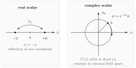
A real scalar with an even potential has the discrete symmetry $\phi\mapsto-\phi$. A complex scalar has a continuous $U(1)$ phase symmetry, equivalently rotations in the $(\phi_1,\phi_2)$ plane.

The Euler–Lagrange equations are obtained by treating $\phi$ and $\phi^*$ as independent fields during variation:

$$\frac{\partial\mathcal L}{\partial\phi^*} -\partial_\mu\frac{\partial\mathcal L}{\partial(\partial_\mu\phi^*)}=0.$$

Since

$$\frac{\partial\mathcal L}{\partial\phi^*}=-m^2\phi, \qquad \frac{\partial\mathcal L}{\partial(\partial_\mu\phi^*)}=\partial^\mu\phi,$$

we get

$$(\Box+m^2)\phi=0.$$

The conjugate equation follows by varying $\phi$:

$$(\Box+m^2)\phi^*=0.$$

The canonical momenta are slightly easy to misread:

$$\pi_\phi=\frac{\partial\mathcal L}{\partial\dot\phi}=\dot\phi^*, \qquad \pi_{\phi^*}=\frac{\partial\mathcal L}{\partial\dot\phi^*}=\dot\phi.$$

So the Hamiltonian density is

$$\mathcal H_{\mathbb C} =\dot\phi^*\dot\phi+\nabla\phi^*\cdot\nabla\phi+m^2\phi^*\phi.$$

In terms of the two real fields, this is just the sum of two real scalar Hamiltonians.

U(1) symmetry and conserved charge

The complex scalar Lagrangian is invariant under a global phase rotation. Fixing an orientation for its Noether generator, choose

$$\phi\longmapsto e^{-i\alpha}\phi, \qquad \phi^*\longmapsto e^{i\alpha}\phi^*,$$

where $\alpha$ is constant. The infinitesimal variations are

$$\delta\phi=-i\alpha\phi, \qquad \delta\phi^*=i\alpha\phi^*.$$

Noether’s theorem gives

$$\begin{aligned} j^\mu &=\frac{\partial\mathcal L}{\partial(\partial_\mu\phi)}\frac{\delta\phi}{\alpha} +\frac{\partial\mathcal L}{\partial(\partial_\mu\phi^*)}\frac{\delta\phi^*}{\alpha} \\ &=-i\phi\,\partial^\mu\phi^*+i\phi^*\partial^\mu\phi. \end{aligned}$$

Thus

$$j^\mu=i\left(\phi^*\partial^\mu\phi-\phi\partial^\mu\phi^*\right).$$

Using the equations of motion,

$$\begin{aligned} \partial_\mu j^\mu &=i\left(\partial_\mu\phi^*\partial^\mu\phi+\phi^*\Box\phi -\partial_\mu\phi\partial^\mu\phi^*-\phi\Box\phi^*\right) \\ &=i\left(\phi^*(-m^2\phi)-\phi(-m^2\phi^*)\right) \\ &=0. \end{aligned}$$

The conserved charge is

$$Q=\int d^3x\,j^0 =i\int d^3x\,\left(\phi^*\dot\phi-\phi\dot\phi^*\right).$$

In real components, with $\pi_i=\dot\phi_i$,

$$Q=\int d^3x\,\left(\phi_2\pi_1-\phi_1\pi_2\right).$$

So electric-type charge is literally angular momentum in the internal two-dimensional field space, up to the orientation convention for the phase rotation.

Noether-generator orientation

This page has oriented its global symmetry as $\phi\to e^{-i\alpha}\phi$. In the gauge-theory convention used later, $D_\mu=\partial_\mu-iqA_\mu$ and $\phi\to e^{iq\alpha}\phi$, so the field written here corresponds to $q=-1$. Interchanging $\phi$ with $\phi^*$, or equivalently sending $\alpha\to-\alpha$, reverses the orientation and flips the signs of $j^\mu$ and $Q$ without changing the spectrum or any physical amplitude.

The sign can be checked directly after quantization. With the unitary rotation

$$U(\alpha)=e^{i\alpha Q},$$

the transformation $U(\alpha)\phi U(\alpha)^\dagger=e^{-i\alpha}\phi$ implies

$$[Q,\phi]=-\phi, \qquad [Q,\phi^\dagger]=+\phi^\dagger.$$

Thus $\phi$ has operator charge $-1$: acting with it lowers the charge of a state by one unit. The particle and antiparticle creation operators below make the corresponding state charges explicit.

Particles and antiparticles of a complex scalar

The real scalar field used one set of oscillators because hermiticity tied the positive- and negative-frequency coefficients together. A complex scalar is not Hermitian. Its positive- and negative-frequency coefficients are independent, and the field expansion contains two oscillator families. After quantization, the classical complex conjugate $\phi^*$ is written as the Hermitian adjoint $\phi^\dagger$:

$$\phi(x)=\int_{\boldsymbol p}\frac{1}{\sqrt{2\omega_{\boldsymbol p}}} \left( a_{\boldsymbol p}e^{-i\omega_{\boldsymbol p}t+i\boldsymbol p\cdot\boldsymbol x} +b_{\boldsymbol p}^\dagger e^{i\omega_{\boldsymbol p}t-i\boldsymbol p\cdot\boldsymbol x} \right),$$

and

$$\phi^\dagger(x)=\int_{\boldsymbol p}\frac{1}{\sqrt{2\omega_{\boldsymbol p}}} \left( a_{\boldsymbol p}^\dagger e^{i\omega_{\boldsymbol p}t-i\boldsymbol p\cdot\boldsymbol x} +b_{\boldsymbol p}e^{-i\omega_{\boldsymbol p}t+i\boldsymbol p\cdot\boldsymbol x} \right),$$

where

$$\int_{\boldsymbol p}\equiv\int\frac{d^3p}{(2\pi)^3}.$$

The nonzero commutators are

$$[a_{\boldsymbol p},a_{\boldsymbol q}^\dagger]=(2\pi)^3\delta^{(3)}(\boldsymbol p-\boldsymbol q), \qquad [b_{\boldsymbol p},b_{\boldsymbol q}^\dagger]=(2\pi)^3\delta^{(3)}(\boldsymbol p-\boldsymbol q).$$

The normal-ordered Hamiltonian is

$$:H: =\int_{\boldsymbol p}\omega_{\boldsymbol p} \left(a_{\boldsymbol p}^\dagger a_{\boldsymbol p}+b_{\boldsymbol p}^\dagger b_{\boldsymbol p}\right).$$

Both particle and antiparticle excitations have positive energy. The charge is

$$:Q: =\int_{\boldsymbol p}\left(a_{\boldsymbol p}^\dagger a_{\boldsymbol p}-b_{\boldsymbol p}^\dagger b_{\boldsymbol p}\right).$$

Thus $a_{\boldsymbol p}^\dagger|0\rangle$ and $b_{\boldsymbol p}^\dagger|0\rangle$ have opposite charges. With the convention above, $a^\dagger$ creates charge $+1$ quanta and $b^\dagger$ creates charge $-1$ quanta.

Indeed, after the harmless vacuum constant is removed by normal ordering,

$$[Q,a_{\boldsymbol p}^\dagger]=a_{\boldsymbol p}^\dagger, \qquad [Q,b_{\boldsymbol p}^\dagger]=-b_{\boldsymbol p}^\dagger.$$

These commutators verify both the relative sign in $Q=N_a-N_b$ and the charge assignment of the two one-particle states.

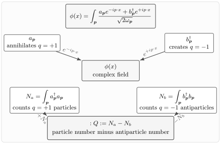
A complex scalar has independent positive- and negative-frequency oscillator families. The field $\phi$ annihilates a charge $+1$ particle through $a_{\boldsymbol p}$ and creates a charge $-1$ antiparticle through $b_{\boldsymbol p}^\dagger$. The conserved charge is $:Q:=N_a-N_b$.

This is the clean field-theoretic interpretation of negative frequencies. They do not describe particles with negative energy. They create antiparticles with positive energy and opposite charge.

The nonrelativistic limit

At low momentum,

$$\omega_{\boldsymbol p}=m+\frac{\boldsymbol p^2}{2m}+O(|\boldsymbol p|^4/m^3).$$

The rest energy $m$ produces rapid time dependence. To isolate slow nonrelativistic motion, write the complex scalar field as

$$\phi(x)=\frac{e^{-imt}}{\sqrt{2m}}\psi(x),$$

where $\psi$ varies slowly compared with $m^{-1}$. This expression keeps the particle sector and drops the antiparticle sector, which is separated by an energy gap of order $2m$.

Substitute into the relativistic Lagrangian

$$\mathcal L_{\mathbb C}=|\dot\phi|^2-|\nabla\phi|^2-m^2|\phi|^2.$$

The time-derivative term gives

$$\dot\phi=\frac{e^{-imt}}{\sqrt{2m}}(\dot\psi-im\psi),$$

so

$$|\dot\phi|^2-m^2|\phi|^2 =\frac{i}{2}\left(\psi^*\dot\psi-\dot\psi^*\psi\right) +\frac{1}{2m}|\dot\psi|^2.$$

The spatial term is

$$-|\nabla\phi|^2=-\frac{1}{2m}\nabla\psi^*\cdot\nabla\psi.$$

Therefore

$$\mathcal L =\frac{i}{2}\left(\psi^*\dot\psi-\dot\psi^*\psi\right) -\frac{1}{2m}\nabla\psi^*\cdot\nabla\psi +\frac{1}{2m}|\dot\psi|^2.$$

The last term is suppressed for slowly varying fields, with $|\dot\psi|\ll m|\psi|$. Dropping it gives

$$\mathcal L_{\mathrm{NR}} =\frac{i}{2}\left(\psi^*\dot\psi-\dot\psi^*\psi\right) -\frac{1}{2m}\nabla\psi^*\cdot\nabla\psi.$$

Up to a total time derivative, this is the usual Schrödinger-field Lagrangian

$$\mathcal L_{\mathrm{NR}} =i\psi^*\dot\psi-\frac{1}{2m}\nabla\psi^*\cdot\nabla\psi.$$

The equation of motion is

$$i\dot\psi=-\frac{\nabla^2}{2m}\psi.$$

The charge density also reduces to the nonrelativistic particle density. Substituting $\phi=e^{-imt}\psi/\sqrt{2m}$ into $j^0=i(\phi^*\dot\phi-\phi\dot\phi^*)$ gives

$$j^0=|\psi|^2+\frac{i}{2m}(\psi^*\dot\psi-\psi\dot\psi^*) .$$

At low energy the second term is suppressed, so

$$Q\simeq\int d^3x\,\psi^*\psi.$$

So the nonrelativistic complex field is the slowly varying envelope left after removing the relativistic rest-energy phase, and its number operator is the low-energy form of the relativistic $U(1)$ charge.

The rest-energy factor is inert under the internal symmetry, so $\psi\to e^{-i\alpha}\psi$. Consequently $[Q,\psi]=-\psi$, exactly as expected for a nonrelativistic annihilation field whose number operator is $Q\simeq\int d^3x\,\psi^*\psi$.

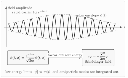
The relativistic field contains a fast carrier phase $e^{-imt}$. The nonrelativistic field $\psi$ is the slowly varying envelope that remains after the rest energy is factored out and antiparticle modes are neglected.

This derivation also explains why nonrelativistic field theory is first order in time while the Klein–Gordon field is second order. The second time derivative is still present in the small correction $|\dot\psi|^2/(2m)$, but it is subleading in the low-energy expansion.

Adding scalar self-interactions

The action principle makes it obvious how to add local interactions. For one real scalar field, the standard quartic theory is

$$\mathcal L =\frac12\partial_\mu\phi\,\partial^\mu\phi -\frac12m^2\phi^2 -\frac{\lambda}{4!}\phi^4.$$

The factor $4!$ is a bookkeeping convention chosen so that four functional derivatives of the interaction bring down a simple factor $\lambda$ in perturbation theory.

The interacting Euler–Lagrange equation is

$$(\Box+m^2)\phi+\frac{\lambda}{3!}\phi^3=0.$$

The plus sign of the nonlinear term follows from writing the potential with a minus sign in $\mathcal L$. For $\lambda\ge 0$, the quartic contribution to the Hamiltonian is nonnegative; a theory with only this quartic interaction and $\lambda<0$ has no stable ground state.

The conjugate momentum is still $\pi=\dot\phi$, and the Hamiltonian is

$$H=H_0+V,$$

with

$$H_0=\int d^3x\,\frac12\left(\pi^2+(\nabla\phi)^2+m^2\phi^2\right),$$

and

$$V=\int d^3x\,\frac{\lambda}{4!}\phi^4.$$

In the Schrödinger picture,

$$i\frac{d}{dt}|\Psi(t)\rangle=(H_0+V)|\Psi(t)\rangle.$$

This is the exact same formal structure as ordinary quantum mechanics, but now $H_0$ describes infinitely many oscillator modes and $V$ couples them. The next page begins the interaction-picture expansion that turns this equation into time-ordered perturbation theory.

For a complex scalar, a derivative-free $U(1)$-preserving quartic interaction is instead

$$\mathcal L_{\mathrm{int}}=-\frac{\lambda}{4}(\phi^*\phi)^2,$$

or with another normalization convention, $-\lambda(\phi^*\phi)^2$. For the displayed $-\lambda(\phi^*\phi)^2/4$ convention, variation with respect to $\phi^*$ gives

$$(\Box+m^2)\phi+\frac{\lambda}{2}(\phi^*\phi)\phi=0.$$

The numerical coefficient changes when the coupling convention changes. More generally, any derivative-free potential $U(\phi^*\phi)$ preserves the phase symmetry and the charge derived above.

At leading order in the nonrelativistic expansion and at tree level, this interaction makes contact with the earlier Bose-gas interaction. With the normalization above,

$$(\phi^*\phi)^2\longrightarrow\frac{(\psi^*\psi)^2}{4m^2},$$

so

$$\mathcal L_{\mathrm{int}}\longrightarrow-\frac{\lambda}{16m^2}(\psi^*\psi)^2.$$

If the nonrelativistic Lagrangian is written as $-g(\psi^*\psi)^2/2$, then this convention gives $g=\lambda/(8m^2)$. Different normalizations of the relativistic quartic simply rescale this matching relation.

Summary

The Klein–Gordon equation is best understood as the Euler–Lagrange equation of a Lorentz-invariant scalar action. For a real scalar, the free Lagrangian is

$$\mathcal L_{\mathbb R}=\frac12(\partial\phi)^2-\frac12m^2\phi^2,$$

with canonical momentum $\pi=\dot\phi$ and positive Hamiltonian density $\frac12\pi^2+\frac12(\nabla\phi)^2+\frac12m^2\phi^2$.

A complex scalar field is equivalent to two real scalars, but it has an extra continuous $U(1)$ symmetry. Noether’s theorem turns that symmetry into a conserved charge. After quantization, the charge counts particles minus antiparticles,

$$:Q:=N_a-N_b,$$

while the Hamiltonian counts the positive energies of both.

The nonrelativistic Schrödinger field emerges from the complex scalar by removing the rest-energy phase $e^{-imt}$ and neglecting antiparticles. The familiar first-order time derivative in the Schrödinger Lagrangian is therefore a low-energy remnant of the relativistic second-order theory.

Finally, the quartic interaction $\lambda\phi^4/4!$ gives the first local interacting scalar field theory. It prepares the way for the interaction picture, Dyson expansion, Wick contractions, and Feynman diagrams.

Common pitfalls

A common mistake is to treat $\phi$ and $\phi^*$ as dependent during variation. In the Euler–Lagrange calculation for a complex field, they are varied independently; the complex conjugation relation is imposed after deriving the equations.

A second normalization mistake is to write $\phi=\phi_1+i\phi_2$ while retaining $\mathcal L_{\mathbb C}=|\partial\phi|^2-m^2|\phi|^2$. That convention gives twice the sum of the canonically normalized real-field actions. Either include $1/\sqrt2$ in the field definition or include $1/2$ in the complex-field Lagrangian.

A third trap is to confuse the $U(1)$ charge with ordinary particle number. For a free complex scalar, $N_a$ and $N_b$ are separately conserved, but the robust symmetry-protected quantity is $Q=N_a-N_b$. Interactions that preserve $U(1)$ can create particle–antiparticle pairs while keeping $Q$ fixed.

A fourth trap is to think that negative-frequency modes are negative-energy particles. In the complex field, the negative-frequency coefficient is an independent creation operator for antiparticles. The Hamiltonian remains positive.

A fifth trap is to miss the total derivative in the nonrelativistic limit. The symmetrized term

$$\frac{i}{2}(\psi^*\dot\psi-\dot\psi^*\psi)$$

and the simpler term $i\psi^*\dot\psi$ differ by a total time derivative, so they give the same classical equations of motion.

A sixth trap is to forget that the nonrelativistic limit of a complex scalar has discarded antiparticle modes. It is valid for processes whose energies are small compared with the pair-production scale $2m$.

Exercises

Exercise 1: Noether current of the complex scalar

For

$$\mathcal L=\partial_\mu\phi^*\partial^\mu\phi-m^2\phi^*\phi,$$

use the infinitesimal transformation

$$\delta\phi=-i\alpha\phi, \qquad \delta\phi^*=i\alpha\phi^*$$

to derive the conserved current.

Solution

The Noether current is

$$j^\mu =\frac{\partial\mathcal L}{\partial(\partial_\mu\phi)}\frac{\delta\phi}{\alpha} +\frac{\partial\mathcal L}{\partial(\partial_\mu\phi^*)}\frac{\delta\phi^*}{\alpha}.$$

Since

$$\frac{\partial\mathcal L}{\partial(\partial_\mu\phi)}=\partial^\mu\phi^*, \qquad \frac{\partial\mathcal L}{\partial(\partial_\mu\phi^*)}=\partial^\mu\phi,$$

we get

$$j^\mu=\partial^\mu\phi^*(-i\phi)+\partial^\mu\phi(i\phi^*).$$

Thus

$$j^\mu=i(\phi^*\partial^\mu\phi-\phi\partial^\mu\phi^*).$$

Using $(\Box+m^2)\phi=0$ and its complex conjugate gives $\partial_\mu j^\mu=0$.

Exercise 2: charge as internal angular momentum

Let

$$\phi=\frac{1}{\sqrt2}(\phi_1+i\phi_2).$$

Show that

$$Q=i\int d^3x\,(\phi^*\dot\phi-\phi\dot\phi^*)$$

is equal to

$$Q=\int d^3x\,(\phi_2\pi_1-\phi_1\pi_2), \qquad \pi_i=\dot\phi_i.$$

Solution

First compute

$$\phi^*\dot\phi =\frac12(\phi_1-i\phi_2)(\dot\phi_1+i\dot\phi_2) =\frac12\left(\phi_1\dot\phi_1+\phi_2\dot\phi_2+i\phi_1\dot\phi_2-i\phi_2\dot\phi_1\right).$$

Similarly,

$$\phi\dot\phi^* =\frac12\left(\phi_1\dot\phi_1+\phi_2\dot\phi_2-i\phi_1\dot\phi_2+i\phi_2\dot\phi_1\right).$$

Subtracting,

$$\phi^*\dot\phi-\phi\dot\phi^* =i(\phi_1\dot\phi_2-\phi_2\dot\phi_1).$$

Therefore

$$i(\phi^*\dot\phi-\phi\dot\phi^*) =\phi_2\dot\phi_1-\phi_1\dot\phi_2.$$

Since $\pi_i=\dot\phi_i$,

$$Q=\int d^3x\,(\phi_2\pi_1-\phi_1\pi_2).$$

This is the angular momentum generator for rotations in the internal $(\phi_1,\phi_2)$ plane, with the orientation fixed by the phase convention.

Exercise 3: nonrelativistic limit of the complex scalar

Set

$$\phi=\frac{e^{-imt}}{\sqrt{2m}}\psi$$

in

$$\mathcal L=|\dot\phi|^2-|\nabla\phi|^2-m^2|\phi|^2.$$

Show that the leading low-energy Lagrangian is

$$\mathcal L_{\mathrm{NR}} =i\psi^*\dot\psi-\frac{1}{2m}\nabla\psi^*\cdot\nabla\psi$$

up to a total derivative.

Solution

The time derivative is

$$\dot\phi=\frac{e^{-imt}}{\sqrt{2m}}(\dot\psi-im\psi).$$

Then

$$|\dot\phi|^2 =\frac{1}{2m}\left(|\dot\psi|^2+m^2|\psi|^2+i m\psi^*\dot\psi-i m\dot\psi^*\psi\right).$$

Also

$$m^2|\phi|^2=\frac{m}{2}|\psi|^2, \qquad |\nabla\phi|^2=\frac{1}{2m}\nabla\psi^*\cdot\nabla\psi.$$

The rest-energy terms cancel, leaving

$$\mathcal L =\frac{i}{2}(\psi^*\dot\psi-\dot\psi^*\psi) -\frac{1}{2m}\nabla\psi^*\cdot\nabla\psi +\frac{1}{2m}|\dot\psi|^2.$$

At low energy, $|\dot\psi|\ll m|\psi|$, so the last term is higher order. Finally,

$$\frac{i}{2}(\psi^*\dot\psi-\dot\psi^*\psi) =i\psi^*\dot\psi-\frac{i}{2}\frac{d}{dt}(\psi^*\psi),$$

so it differs from $i\psi^*\dot\psi$ only by a total derivative. Hence

$$\mathcal L_{\mathrm{NR}} =i\psi^*\dot\psi-\frac{1}{2m}\nabla\psi^*\cdot\nabla\psi.$$

Exercise 4: dimension of the quartic coupling

In $d$ spacetime dimensions, determine the mass dimension of a real scalar field and of the coupling $\lambda$ in

$$\mathcal L_{\mathrm{int}}=-\frac{\lambda}{4!}\phi^4.$$

For which $d$ is $\lambda$ dimensionless?

Solution

The action is dimensionless, so $\mathcal L$ has mass dimension $d$. The kinetic term has dimension

$$[\partial_\mu\phi\partial^\mu\phi]=2+2[\phi].$$

Thus

$$2+2[\phi]=d,$$

so

$$[\phi]=\frac{d-2}{2}.$$

The interaction term has dimension

$$[\lambda]+4[\phi]=d.$$

Therefore

$$[\lambda]=d-4\left(\frac{d-2}{2}\right)=4-d.$$

The quartic coupling is dimensionless in

$$d=4.$$

This is why $\phi^4$ theory in four spacetime dimensions is the standard marginal scalar interaction by power counting.

References and further reading

• Mark Srednicki, Quantum Field Theory, Sections 3 and 22, for canonical scalar fields and continuous symmetries.
• Steven Weinberg, The Quantum Theory of Fields, Volume I, Chapters 5 and 7, for scalar fields, antiparticles, and the canonical formalism.
• Sidney Coleman, Lectures of Sidney Coleman on Quantum Field Theory, Chapters 3 and 6, for scalar fields and internal symmetries.
• A. Zee, Quantum Field Theory in a Nutshell, Chapters I.4, I.8, and III.5, for physical motivation, canonical quantization, and nonrelativistic field theory.