Thresholds, Cuts, and Imaginary Parts

The spectral representation says that a propagator has isolated poles when a field creates stable particles and cuts when it creates continua. This page explains what those cuts look like near their thresholds and why their discontinuities are imaginary parts. The simplest calculation is not a full relativistic loop integral. It is the nonrelativistic expansion of the particles that are just barely allowed to go on shell.

The key point is that a threshold is controlled by long times and small relative momenta. Near the opening of an $n$-particle channel, each particle is almost at rest in the center-of-momentum frame, so

$$\omega_{\mathbf p}=\sqrt{\mathbf p^2+m^2} =m+{\mathbf p^2\over2m}+\cdots.$$

The rest masses determine where the branch point sits. The Gaussian integrals over the small relative momenta determine the power of the branch cut. This is one of the cleanest places where analytic structure, phase space, and time evolution become the same statement in different languages.

A practical threshold calculation has three steps.

1. Identify the lightest intermediate state in the channel and subtract its rest energy.
2. Expand the on-shell energies for small relative momenta.
3. Count the remaining relative-momentum phase space, including constraints and possible angular-momentum or symmetry suppressions.

The third step is where many mistakes happen. The exponent is not determined by the number of particles alone; it is determined by the number of independent soft variables that can actually appear in the channel.

Thresholds from long-time propagation

Nonrelativistic resolvent normalization

On this page we often use a nonrelativistic Green function without the overall Feynman factor $i$:

$$G_0(\omega,\mathbf p)={1\over \omega-\epsilon_{\mathbf p}+i0}, \qquad \epsilon_{\mathbf p}={\mathbf p^2\over2m}.$$

With the fully relativistic convention used earlier, the scalar Feynman propagator is $i/(p^2-m^2+i0)$. The location of poles, the threshold powers, and the discontinuities are independent of this bookkeeping choice; only a few overall signs and factors of $i$ move around.

Consider an intermediate state made from three identical massive particles. In the center-of-momentum frame and close to threshold, write the total energy as

$$\omega=3m+E, \qquad E\ll m.$$

The three momenta satisfy

$$\mathbf p_1+\mathbf p_2+\mathbf p_3=0,$$

so there are only two independent relative momenta. The total energy above threshold is quadratic:

$$E={\mathbf p_1^2+\mathbf p_2^2+\mathbf p_3^2\over2m}+O(\mathbf p^4/m^3).$$

After a linear change of variables to two relative momenta $\mathbf q$ and $\mathbf r$, this becomes

$$E={\mathbf q^2+\mathbf r^2\over2\mu_{\rm red}}$$

after rescaling the two Jacobi momenta to a common reduced-mass parameter $\mu_{\rm red}$. Its precise normalization is not important for the analytic power; what matters is that the threshold problem is a six-dimensional Gaussian integral.

In the time domain, the threshold part of a self-energy has the schematic form

$$\Sigma(t)\sim e^{-3imt} \int d^3q\,d^3r\, \exp\left[-i{\mathbf q^2+\mathbf r^2\over2\mu_{\rm red}}t\right].$$

For large $t$, each three-dimensional Gaussian contributes a factor $t^{-3/2}$. Therefore

$$\boxed{ \Sigma(t)\sim {e^{-3imt}\over t^3} \qquad (t\to\infty). }$$

The $e^{-3imt}$ factor knows the threshold energy. The power $t^{-3}$ knows the number of independent soft momenta. This is a beautifully economical way to read the branch point before doing any detailed loop integral.

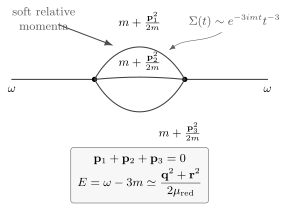
Near the three-particle threshold, the internal particles are almost on shell and almost at rest in the center-of-momentum frame. The two independent relative momenta give a six-dimensional Gaussian integral, so the long-time behavior is $e^{-3imt}/t^3$.

Now Fourier transform the large-time tail. Up to terms analytic in $E=\omega-3m$, the relevant integral is

$$\int_0^\infty dt\,{e^{i(E+i0)t}\over t^3}.$$

This integral is ultraviolet divergent at $t=0$, because the large-time approximation is not valid at short times. That divergence produces analytic local terms. The nonanalytic part is unambiguous. By analytic continuation of

$$\int_0^\infty dt\,t^{\alpha-1}e^{i(E+i0)t} =\Gamma(\alpha)\big[-i(E+i0)\big]^{-\alpha},$$

and continuing to the integer case where logarithms appear, one obtains

$$\boxed{ \Sigma_{\rm nonan}(\omega) = C\, (\omega-3m)^2 \log\left[-{\omega-3m+i0\over\Lambda}\right]+\text{analytic terms}. }$$

Here $C$ is a real constant depending on the vertices and normalizations, and $\Lambda$ is an arbitrary reference scale introduced when separating the logarithm from analytic counterterms. The important part is the structure

$$(\omega-3m)^2\log(\omega-3m).$$

A logarithm has a branch cut. Thus the three-particle continuum turns the self-energy into a multi-valued function of energy.

Phase space and the power of a threshold

The same power follows from counting phase space. Define the nonrelativistic $n$-particle density of states at fixed total momentum by

$$\rho_n(E) \propto \int \prod_{a=1}^n d^3p_a\, \delta^{(3)}\left(\sum_{a=1}^n\mathbf p_a\right) \delta\left(E-\sum_{a=1}^n{\mathbf p_a^2\over2m_a}\right).$$

After the total-momentum delta function is used, there are $3(n-1)$ relative momentum variables. The remaining energy delta function fixes the radius of a sphere in this relative-momentum space. Hence, for small positive $E$,

$$\boxed{ \rho_n(E)\propto E^{\frac{3(n-1)}{2}-1}\theta(E) =E^{\frac{3n-5}{2}}\theta(E). }$$

For two particles,

$$\rho_2(E)\propto E^{1/2}\theta(E),$$

so two-particle thresholds in four spacetime dimensions usually have square-root branch points. For three particles,

$$\rho_3(E)\propto E^2\theta(E),$$

which matches the discontinuity of $E^2\log(-E-i0)$.

This counting assumes an $s$-wave threshold and a matrix element that is nonzero at zero relative momentum. If a symmetry or angular-momentum selection rule forces the matrix element to vanish like $q^\ell$, the threshold acquires extra powers. This is why the phase-space exponent is the starting point, not always the final answer.

More explicitly, for $E>0$,

$$\log[-(E+i0)]=\log E-i\pi,$$

so

$$\operatorname{Im}\Sigma(E+i0) =-\pi C E^2\theta(E)$$

up to the overall convention contained in $C$. The discontinuity is

$$\operatorname{Disc}\Sigma(E) =\Sigma(E+i0)-\Sigma(E-i0) =-2\pi i C E^2\theta(E).$$

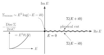
The variable $E=\omega-3m$ measures energy above threshold. The amplitude is analytic away from the cut. For a three-particle threshold in four spacetime dimensions, the discontinuity begins as $E^2\theta(E)$.

This is the local form of a general statement: imaginary parts begin when intermediate states can go on shell. Below threshold, the energy-conserving delta functions cannot be satisfied. Above threshold, they can, and the amplitude develops a discontinuity.

The golden rule from time evolution

The previous discussion was analytic. The same imaginary part appears in ordinary time-dependent perturbation theory as a transition rate.

Let

$$H=H_0+V,$$

and let $|i\rangle$, $|f\rangle$ be eigenstates of $H_0$ with energies $E_i$ and $E_f$. In the interaction picture, the first-order transition amplitude over a long time interval is

$$A_{fi}^{(1)} = -i\int_{-T/2}^{T/2}dt\, \langle f|V_I(t)|i\rangle.$$

Since

$$V_I(t)=e^{iH_0t}Ve^{-iH_0t},$$

we get

$$A_{fi}^{(1)} =-iV_{fi}\int_{-T/2}^{T/2}dt\,e^{i(E_f-E_i)t} =-iV_{fi}\,{2\sin[(E_f-E_i)T/2]\over E_f-E_i}.$$

As $T\to\infty$,

$$\int_{-T/2}^{T/2}dt\,e^{i(E_f-E_i)t} \longrightarrow 2\pi\delta(E_f-E_i),$$

so the amplitude becomes

$$A_{fi}^{(1)} \longrightarrow -2\pi i\,\delta(E_f-E_i)V_{fi}.$$

Squaring the amplitude produces the familiar factor

$$[2\pi\delta(E_f-E_i)]^2 =2\pi T\,\delta(E_f-E_i),$$

because $2\pi\delta(0)=T$. Dividing by $T$ gives Fermi’s golden rule:

$$\boxed{ d\Gamma_{i\to f}=2\pi |V_{fi}|^2\delta(E_f-E_i)\,d\nu_f, }$$

where $d\nu_f$ is the final-state density of states.

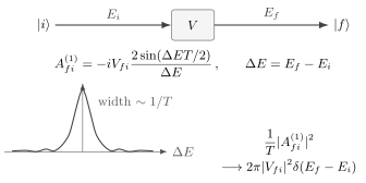
For finite time $T$, the squared transition amplitude contains a narrow peak of width $1/T$. As $T\to\infty$, the peak becomes an energy-conserving delta function, and its area grows like $T$, producing a transition probability per unit time.

The golden rule is the real-time ancestor of the cutting rule. The delta function in energy is not a formal trick. It says that a transition rate exists only when the final particles can be real particles satisfying energy conservation.

The same finite-time derivation also explains why a decay width is an imaginary part of an energy. The transition probability initially grows as $P_{\rm decay}(t)\simeq\Gamma t$, which is the short-time expansion of $1-e^{-\Gamma t}$; equivalently, the survival probability is $P_{\rm surv}(t)\simeq1-\Gamma t$, the first terms of $e^{-\Gamma t}$. The survival amplitude decays as $e^{-\Gamma t/2}$. In frequency space, exponential decay means that the pole has moved off the real axis. This is the real-time version of the branch-cut story.

Imaginary parts and on-shell intermediate states

Let $S=1+iT$. Unitarity, $S^\dagger S=1$, implies

$$-i(T-T^\dagger)=T^\dagger T.$$

Between states $|i\rangle$ and $|f\rangle$, and after inserting a complete set of intermediate states,

$$-i\left(T_{fi}-T^*_{if}\right) =\sum_n T^*_{nf}T_{ni}.$$

For forward scattering, $f=i$, this becomes

$$\boxed{ 2\operatorname{Im}T_{ii}=\sum_n |T_{ni}|^2. }$$

With the usual momentum-conserving delta functions and relativistic phase-space measures restored, this is the optical theorem. Its diagrammatic version says that the discontinuity of a graph is obtained by cutting internal lines and putting the cut particles on shell. For a scalar line, the schematic replacement is

$${1\over k^2-m^2+i0} \quad\leadsto\quad -2\pi i\,\theta(k^0)\delta(k^2-m^2)$$

inside a discontinuity. The precise sign depends on the overall amplitude convention, but the physical content is invariant: a cut line is a real intermediate particle.

This explains why ultraviolet counterterms do not determine imaginary parts. Counterterms are local polynomials in momenta, while imaginary parts across physical cuts are nonlocal and fixed by phase space. Local terms can shift masses, residues, and subtraction constants; they cannot manufacture the phase-space branch cut of real intermediate states.

Nonrelativistic Green functions with a potential

The same ideas are useful in the simplest nonrelativistic field theory. Let

$$\mathcal L =\psi^\dagger\left(i\partial_t+{\nabla^2\over2m}\right)\psi -u(\mathbf x)\psi^\dagger\psi.$$

The free Green function in frequency-momentum space is

$$G_0(\omega,\mathbf p) ={1\over\omega-\epsilon_{\mathbf p}+i0}, \qquad \epsilon_{\mathbf p}={\mathbf p^2\over2m}.$$

The potential is an interaction vertex

$$V=\int d^3x\,u(\mathbf x)\psi^\dagger(\mathbf x)\psi(\mathbf x),$$

with momentum-space matrix element

$$U(\mathbf p',\mathbf p) =\int d^3x\,e^{-i(\mathbf p'-\mathbf p)\cdot\mathbf x}u(\mathbf x).$$

Expanding the exact Green function gives the Born series

$$\begin{aligned} G(\omega;\mathbf p',\mathbf p) &=(2\pi)^3\delta^{(3)}(\mathbf p'-\mathbf p)G_0(\omega,\mathbf p)\\ &\quad+G_0(\omega,\mathbf p')U(\mathbf p',\mathbf p)G_0(\omega,\mathbf p)+\cdots. \end{aligned}$$

Equivalently,

$$G=G_0+G_0UG_0+G_0UG_0UG_0+\cdots.$$

The next page will reorganize this expansion in terms of the $T$-matrix,

$$T=U+UG_0U+UG_0UG_0U+\cdots,$$

but already here the analytic structure is visible. Each free propagator contributes a pole. Integrating over intermediate momenta can turn a pole into a cut when a continuum of intermediate energies becomes available.

Double poles and secular terms

A final lesson from the nonrelativistic Green function is worth isolating. Suppose a perturbative correction to a one-particle propagator produces

$$G(\omega) ={1\over\omega-\epsilon+i0} +{\delta\epsilon\over(\omega-\epsilon+i0)^2}+\cdots.$$

The second term has a double pole. With the Fourier convention used here, for $t>0$,

$$\int{d\omega\over2\pi}\,{e^{-i\omega t}\over(\omega-\epsilon+i0)^2} =-t e^{-i\epsilon t}.$$

Thus the order-$\delta\epsilon$ correction is $-\delta\epsilon\,t e^{-i\epsilon t}$. This growing polynomial factor is called a secular term. It is not a physical growth of probability; together with the free transform $-i e^{-i\epsilon t}$ it is precisely the first-order Taylor expansion of a shifted frequency:

$$-i e^{-i(\epsilon+\delta\epsilon)t} =-i e^{-i\epsilon t}-\delta\epsilon\,t e^{-i\epsilon t}+\cdots.$$

Thus a double pole in fixed-order perturbation theory is often telling us to resum the expansion and move the pole:

$${1\over\omega-\epsilon+i0} +{\delta\epsilon\over(\omega-\epsilon+i0)^2}+\cdots \approx {1\over\omega-\epsilon-\delta\epsilon+i0}.$$

If $\operatorname{Im}\delta\epsilon<0$, the shifted pole gives exponential decay or damping; a positive imaginary part would instead produce growth and signal an instability or a sign error in a supposedly stable problem. If $\delta\epsilon$ is real, it gives an energy shift. Either way, the analytic structure of the Green function is the most compact way to summarize long-time physics.

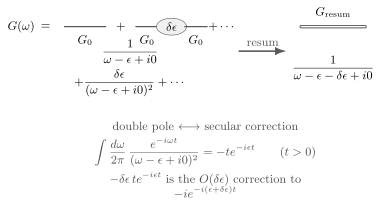
Expanding around an unperturbed pole creates higher-order poles. In time, a double pole gives a secular term proportional to $t e^{-i\epsilon t}$. Resumming the self-energy moves the pole instead of leaving an expansion that grows at late times.

Summary

A threshold is the point where a new class of intermediate states can satisfy energy-momentum conservation. Near threshold, the particles are slow in the center-of-momentum frame, so the analytic behavior is determined by nonrelativistic phase space. For $n$ massive particles in four spacetime dimensions,

$$\rho_n(E)\propto E^{(3n-5)/2}\theta(E), \qquad E=\omega-\sum_a m_a.$$

For a three-particle threshold this gives $E^2\theta(E)$ as the discontinuity and $E^2\log(-E-i0)$ as the corresponding nonanalytic part of the self-energy.

Imaginary parts are not mysterious. In real time, they are transition probabilities per unit time. In momentum space, they are discontinuities across cuts. In diagrams, they arise when internal lines can be cut and placed on shell. This is the first practical form of unitarity in perturbation theory.

The same mechanism also explains why perturbation theory develops double poles near shifted one-particle energies. A double pole corresponds to a secular term in time; resummation turns that secular term into a shifted or broadened pole. This logic prepares the scattering and Dyson-resummation discussion that follows.

Common pitfalls

Calling every nonanalyticity a pole. A stable particle gives a pole. A continuum gives a branch cut. They have different time-domain signatures: a pole gives a pure exponential, while a cut gives an integral over exponentials and usually a power-law prefactor.

Forgetting the center-of-momentum constraint. For an $n$-particle threshold at fixed total momentum, there are $3(n-1)$ relative momentum variables, not $3n$ independent ones.

Treating the logarithm as unique. The expression $E^2\log(-E-i0)$ is defined up to analytic terms such as constants, $E$, and $E^2$. Those analytic terms are local and convention-dependent; the discontinuity is physical.

Squaring a delta function too casually. The rule $[2\pi\delta(E)]^2=2\pi T\delta(E)$ is a shorthand for a finite-time limit. The extra factor of $T$ is why a probability becomes a rate.

Confusing a cut with a Cauchy contour cut. A branch cut in the complex plane records multi-valued analytic behavior. A diagrammatic cut records on-shell intermediate states. They are related by unitarity, but they are not the same piece of notation.

Forgetting selection rules at threshold. Phase space gives the default power. If the amplitude vanishes at threshold because of angular momentum, parity, or an internal symmetry, the discontinuity starts with additional powers of $E$.

Exercises

Exercise 1

Derive the near-threshold scaling of the fixed-total-momentum $n$-particle phase space in three spatial dimensions:

$$\rho_n(E)\propto E^{(3n-5)/2}\theta(E).$$

Solution

Start from

$$\rho_n(E) \propto \int \prod_{a=1}^n d^3p_a\, \delta^{(3)}\left(\sum_{a=1}^n\mathbf p_a\right) \delta\left(E-\sum_{a=1}^n{\mathbf p_a^2\over2m_a}\right).$$

Use the momentum-conservation delta function to remove three variables. This leaves

$$d=3(n-1)$$

relative momentum variables. After a nonsingular linear transformation, the quadratic energy becomes a sum of squares,

$$\sum_{a=1}^n{\mathbf p_a^2\over2m_a}=\sum_{j=1}^d c_j Q_j^2,$$

with positive coefficients $c_j$. Rescaling the $Q_j$ absorbs the $c_j$ into an overall constant, so the scaling is

$$\rho_n(E)\propto\int d^dQ\,\delta(E-Q^2).$$

In $d$-dimensional spherical coordinates,

$$\int d^dQ\,\delta(E-Q^2) \propto \int_0^\infty dR\,R^{d-1}\delta(E-R^2).$$

Using $\delta(E-R^2)=\delta(R-\sqrt E)/(2\sqrt E)$ for $E>0$, we get

$$\rho_n(E)\propto E^{d/2-1}\theta(E).$$

Since $d=3(n-1)$,

$$\rho_n(E)\propto E^{3(n-1)/2-1}\theta(E) =E^{(3n-5)/2}\theta(E).$$

Exercise 2

Show that a time-domain tail

$$F(t)\sim {e^{-iE_{\rm th}t}\over t^\alpha}$$

produces a branch point at $\omega=E_{\rm th}$. For noninteger $\alpha$, find the nonanalytic power of $\omega-E_{\rm th}$.

Solution

The singular part of the Fourier transform is governed by

$$I(E)=\int_0^\infty dt\,t^{-\alpha}e^{i(E+i0)t}, \qquad E=\omega-E_{\rm th}.$$

For noninteger $\alpha$, analytic continuation of the half-line transform gives

$$I(E)=\Gamma(1-\alpha)\big[-i(E+i0)\big]^{\alpha-1},$$

up to analytic terms if the small-$t$ region requires subtraction. The phase multiplying this expression is fixed by the phase of the original long-time tail. For a real-analytic Green function with its physical cut at $E>0$, it is conventional to display the nonanalytic part as

$$I_{\rm nonan}(E)\propto \big[-(E+i0)\big]^{\alpha-1}.$$

A noninteger power is multi-valued and has its cut for $E>0$, so it has a branch point at $E=0$, or $\omega=E_{\rm th}$. When $\alpha$ is an integer, the pole of $\Gamma(1-\alpha)$ converts the power into a logarithm. For example, $\alpha=3$ gives

$$I_{\rm nonan}(E)\propto E^2\log(-E-i0)$$

up to the choice of branch and analytic terms.

Exercise 3

Starting from the finite-time first-order amplitude

$$A_{fi}^{(1)}=-iV_{fi}{2\sin(\Delta E T/2)\over\Delta E}, \qquad \Delta E=E_f-E_i,$$

derive Fermi’s golden rule.

Solution

The transition probability into a set of final states is

$$dP=|V_{fi}|^2 {4\sin^2(\Delta E T/2)\over(\Delta E)^2}\,d\nu_f.$$

As a distribution,

$$\lim_{T\to\infty}{1\over T}{4\sin^2(\Delta E T/2)\over(\Delta E)^2} =2\pi\delta(\Delta E).$$

This can be checked by integrating against a smooth test function and changing variables $x=\Delta E T/2$. Dividing by $T$ gives the transition rate

$$d\Gamma={dP\over T} =2\pi |V_{fi}|^2\delta(E_f-E_i)d\nu_f.$$

The delta function enforces energy conservation, while $d\nu_f$ supplies the density of final states.

Exercise 4

Use the distribution identity

$${1\over x+i0}=\operatorname{PV}{1\over x}-i\pi\delta(x)$$

to compute the imaginary part of the second-order energy shift

$$\Delta E_i^{(2)} =\sum_n {|V_{ni}|^2\over E_i-E_n+i0}.$$

Interpret the result.

Solution

Apply the identity with $x=E_i-E_n$:

$$\Delta E_i^{(2)} = \sum_n |V_{ni}|^2\operatorname{PV}{1\over E_i-E_n} -i\pi\sum_n |V_{ni}|^2\delta(E_i-E_n).$$

Thus

$$\operatorname{Im}\Delta E_i^{(2)} =-\pi\sum_n |V_{ni}|^2\delta(E_i-E_n).$$

If the state $|i\rangle$ can decay into the states $|n\rangle$, its amplitude behaves as

$$e^{-i(E_i+\Delta E_i)t} =e^{-i(E_i+\operatorname{Re}\Delta E_i)t} e^{\operatorname{Im}\Delta E_i\, t}.$$

A negative imaginary part gives decay. The decay rate is

$$\Gamma_i=-2\operatorname{Im}\Delta E_i^{(2)} =2\pi\sum_n |V_{ni}|^2\delta(E_i-E_n),$$

which is Fermi’s golden rule. The real principal-value part is the energy shift.

Exercise 5

Show that a correction

$$G(\omega)=G_0(\omega)+\delta\epsilon\,G_0(\omega)^2+\cdots, \qquad G_0(\omega)={1\over\omega-\epsilon+i0},$$

is the first two terms in the expansion of a propagator with a shifted pole.

Solution

A shifted pole has

$$G_{\rm shifted}(\omega) ={1\over\omega-\epsilon-\delta\epsilon+i0}.$$

Expanding for small $\delta\epsilon$ gives

$$G_{\rm shifted}(\omega) ={1\over\omega-\epsilon+i0} {1\over 1-\delta\epsilon/(\omega-\epsilon+i0)}.$$

Using $1/(1-x)=1+x+\cdots$,

$$G_{\rm shifted}(\omega) ={1\over\omega-\epsilon+i0} +{\delta\epsilon\over(\omega-\epsilon+i0)^2}+\cdots.$$

Thus the double pole is not a new particle. It is the perturbative expansion of the shifted one-particle pole.

References and further reading

• Mark Srednicki, Quantum Field Theory, sections 14, 15, and 25, for self-energies, spectral representations, and unstable particles.
• Sidney Coleman, Lectures on Quantum Field Theory, chapters 15–17, for spectral representations, self-energy singularities, Breit–Wigner behavior, and decay laws.
• A. Zee, Quantum Field Theory in a Nutshell, chapter III.8, for a concise explanation of imaginary parts, unitarity, and Cutkosky cuts.
• Steven Weinberg, The Quantum Theory of Fields, vol. I, sections 3.6, 10.7, and 10.8, for unitarity, spectral representations, and dispersion relations.