Monopoles and Confinement in Three-Dimensional Gauge Theory

The previous pages studied instantons in the two-dimensional $O(3)$ sigma model. Those instantons were finite-action maps between spheres, and their effects were invisible in ordinary perturbation theory. This page turns to a gauge-theory version of the same lesson: in three Euclidean dimensions, monopoles are instantons.

The result is one of the cleanest analytic mechanisms for confinement. A weakly coupled theory can have massive charged particles, an apparently harmless unbroken $U(1)$ gauge field, and yet an external probe with odd center charge cannot be isolated in the infrared. The reason is not a perturbative photon diagram. It is a gas of monopole instantons. Their long-range Coulomb fields form a plasma, the plasma Debye-screens the dual magnetic field, and the unscreened Wilson loop acquires an area law.

We use the weakly coupled three-dimensional adjoint-Higgs model with a massive neutral Higgs as well as massive charged vectors. Below both heavy masses, its regulated dilute monopole gas gives a compact dual scalar, a nonperturbative mass and a string tension for unscreened probes. This is a semiclassical effective calculation; the later four-dimensional comparison is an analogy, not a derivation of QCD confinement.

Required background. Theta angle and instanton corrections introduces dilute instanton sums, fugacity, and the plasma language used here.

Helpful background. Confinement and screening in two-dimensional QED distinguishes an area law from screening and string breaking, while dimensional transmutation and mass gaps reviews nonperturbatively generated scales. The mechanism has three layers: broken $SU(2)$ supplies a nonsingular monopole core and a weakly coupled long-distance photon; compactness requires monopole and anti-monopole events; and their grand canonical gas maps to a sine-Gordon theory for a compact dual photon. The resulting mass gap is generated dynamically, and its Wilson-loop area law is not ordinary Yukawa screening.

The SU(2) model and the monopole instanton

Normalization. We work in three Euclidean dimensions with coordinates $x^\nu$, $\nu=1,2,3$, and

$$\epsilon_{123}=+1.$$

Write the compact Abelian connection as $a_\mu$, distinct from the non-Abelian connection $A_\mu^a$ below, and normalize a charge-one loop as $\exp(i\oint a)$. Then

$$S_{\rm Max}[a]={1\over4e^2}\int d^3x\,f_{\mu\nu}f_{\mu\nu} ={1\over2e^2}\int d^3x\,B_\mu B_\mu,$$

where

$$B_\mu={1\over2}\epsilon_{\mu\nu\rho}f_{\nu\rho},\qquad f=da \quad\text{locally outside monopole cores}.$$

In three dimensions $e^2$ has dimensions of mass. A unit monopole has magnetic flux

$$\int_{S^2} B_\mu\,dS_\mu=2\pi.$$

This fixes the numerical coefficients of Maxwell duality. The core prescription determines the fugacity and higher corrections, rather than changing the Gaussian coefficients at fixed normalization.

For the broken $SU(2)$ ultraviolet completion, take $g_3^2>0$, $v>0$ and rescale the microscopic fields so that the action has an overall factor $1/g_3^2$. Then

$$[g_3^2]=[v]=1, \qquad m_W=v\quad\text{at tree level}.$$

Use Hermitian generators $T^a=\sigma^a/2$ and the rescaled connection $D=\partial-iA^aT^a$. Thus the adjoint derivative and curvature are

$$\begin{aligned} (D_\mu\phi)^a&=\partial_\mu\phi^a+\epsilon^{abc}A_\mu^b\phi^c,\\ F_{\mu\nu}^a&=\partial_\mu A_\nu^a-\partial_\nu A_\mu^a +\epsilon^{abc}A_\mu^bA_\nu^c. \end{aligned}$$

In unitary gauge, with $\phi^a\to v\delta^{a3}$, choose

$$a_\mu=-{A_\mu^3\over2},\qquad Q_{\rm e}=-2T^3, \qquad D_\mu=\partial_\mu-iQ_{\rm e}a_\mu.$$

The two fundamental weights have charges $\pm1$, and the massive adjoint $W$ bosons have charges $\pm2$. Setting the massive $W$ backgrounds to zero gives $F^3=-2f$; substituting this into the microscopic gauge action yields the tree-level matching

$${(F^3)^2\over4g_3^2}={f^2\over g_3^2} ={f^2\over4e^2},\qquad e^2={g_3^2\over4}.$$

Below the heavy thresholds, $e^2$ means the matched low-energy coefficient, with perturbative threshold corrections if retained. These charge conventions determine both magnetic orientation and which electric strings can break.

A convenient ultraviolet completion is the three-dimensional Georgi–Glashow model, with the rescaled Euclidean action

$$S_E={1\over g_3^2}\int d^3x\, \left[ {1\over4}(F_{\mu\nu}^a)^2 +{1\over2}(D_\mu\phi^a)^2 +V(\phi^a\phi^a) \right].$$

In the rescaled-field convention, one possible potential is

$$V(\phi^2) ={\kappa\over4}(\phi^2-v^2)^2,\qquad \kappa={\lambda\over g_3^2}>0,$$

where $\kappa$ is dimensionless. Expanding $\phi^3=v+H$ and comparing the quadratic potential with the kinetic term gives $m_H^2=2\kappa v^2$ at tree level.

The potential is chosen so that

$$\phi^a\phi^a\to v^2$$

far from the origin. A vacuum expectation value of an adjoint field breaks

$$SU(2)\longrightarrow U(1).$$

The charged gauge bosons become massive while the Abelian photon remains massless in perturbation theory. A photon-only effective description requires distances large compared with both $m_W^{-1}$ and $m_H^{-1}$. We use

$${v\over g_3^2}\gg1,\qquad m_\gamma\ll m_H,m_W,$$

with fixed positive $\kappa$ in a perturbatively controlled regime. The nonperturbative $m_\gamma$ will be obtained below; the hierarchy can then be checked. The exactly vanishing-$\kappa$ BPS limit is useful for the isolated classical action but leaves a massless neutral scalar, so it does not justify this photon-only truncation.

The nonperturbative object is the finite-action monopole configuration. At spatial infinity the scalar field defines a map

$$S^2_\infty\longrightarrow SU(2)/U(1)\simeq S^2,$$

and such maps are classified by

$$\pi_2(S^2)=\mathbb Z.$$

The charge-one configuration can be represented by the hedgehog ansatz

$$\phi^a(x)=v\,h(r){x^a\over r}, \qquad A_\mu^a(x)={1-k(r)\over r^2}\epsilon_{a\mu b}x^b, \qquad r=\sqrt{x_\mu x_\mu}.$$

The profile functions satisfy

$$h(0)=0, \qquad k(0)=1, \qquad h(\infty)=1, \qquad k(\infty)=0.$$

The epsilon order is consequential. For $n^a=x^a/r$ and $k=0$,

$$\partial_\mu\mathbf n={\mathbf e_\mu-n_\mu\mathbf n\over r},\qquad \mathbf A_\mu\times\mathbf n =-{\mathbf e_\mu-n_\mu\mathbf n\over r},$$

so $D_\mu\mathbf n=0$ asymptotically. Reversing the epsilon indices would add these terms instead of canceling them. More generally, with $\mathbf n=\boldsymbol\phi/|\boldsymbol\phi|$, define the gauge-invariant projected curvature where $|\phi|\ne0$ by

$$\mathcal F_{\mu\nu} =\mathbf n\cdot\mathbf F_{\mu\nu} -\mathbf n\cdot(D_\mu\mathbf n\times D_\nu\mathbf n), \qquad f_{\mu\nu}=-{1\over2}\mathcal F_{\mu\nu}.$$

For the positive Higgs hedgehog, direct evaluation at large radius gives

$$\mathcal B_\mu\equiv{1\over2}\epsilon_{\mu\nu\rho}\mathcal F_{\nu\rho} =-{x_\mu\over r^3},\qquad B_\mu={x_\mu\over2r^3},\qquad \int_{S^2}\mathbf B\cdot d\mathbf S=2\pi.$$

Thus positive Higgs degree has negative projected non-Abelian flux but positive flux in our explicitly defined Abelian connection. The adjoint definitions and asymptotic solution are in ’t Hooft 1974, pp. 279–281, Eqs. (2.2), (2.15)–(2.20), PDF; the fundamental half-isospin probe is discussed on ’t Hooft 1974, p. 283, PDF. His gauge field is related by $A=eW$ before our Abelian minus-half map; the source’s magnetic-dual orientation must also be translated when comparing its outward field.

The core itself is nonsingular because the non-Abelian fields and vanishing Higgs magnitude resolve the Abelian singularity. The Abelian projection is not a smooth coordinate description at $\phi=0$. Inspect the outward Abelian arrows in the schematic section below:

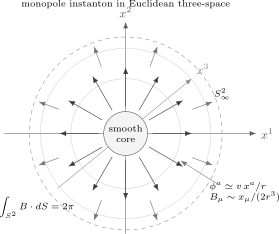
Schematic section through a three-dimensional monopole core, not a profile solution. For $\phi^a\simeq vx^a/r$ the projected non-Abelian flux is $-4\pi$; $f=-\mathcal F/2$ gives the outward Abelian flux $+2\pi$ shown. In unitary gauge this is $a=-A^3/2$. The photon-only regime lies outside both heavy Compton lengths.

Why call this an instanton? In three Euclidean dimensions it is localized in all three coordinates. If one later interprets one coordinate as imaginary time, the monopole is an event: it changes the magnetic flux of the two-dimensional spatial slice. Equivalently, the topological current

$$j_m^\mu={1\over2\pi}B^\mu$$

would be conserved in noncompact Maxwell theory,

$$\partial_\mu j_m^\mu=0,$$

but monopole events violate this conservation law by integer amounts:

$$\partial_\mu B_\mu=2\pi\sum_i q_i\delta^{(3)}(x-x_i), \qquad q_i\in\mathbb Z.$$

This is the gauge-theory analogue of an instanton changing a winding number.

The action of a single monopole has the form

$$S_0={4\pi v\over g_3^2}\,C\!\left({\lambda\over g_3^2}\right),$$

where $C$ is determined by the dimensionless scalar coupling; its detailed profile dependence is not computed here. In the BPS limit $\kappa=0$, completing the square with $B_\mu^a=\epsilon_{\mu\nu\rho}F_{\nu\rho}^a/2$ gives

$$S_E={1\over2g_3^2}\int d^3x\,(B_\mu^a+D_\mu\phi^a)^2 -{1\over g_3^2}\int_{S^2_\infty}\phi^a B_\mu^a\,dS_\mu \ge {4\pi v\over g_3^2}$$

for this positive-degree hedgehog. Saturation has $B^a=-D\phi^a$ and $C(0)=1$; it does not supply the missing neutral mass at $\kappa=0$. At positive $\kappa$, the core action remains large. Since a fugacity is a weight per unit three-volume, write it dimensionally as

$$\zeta=\mathcal A(v,g_3^2,\lambda)e^{-S_0}, \qquad [\mathcal A]=[\zeta]=3,$$

where the prefactor $\mathcal A$ contains zero-mode Jacobians, the one-loop determinant, and powers of the core scales. The exponential is universal at leading semiclassical order; the prefactor is not simply a dimensionless constant.

From isolated monopoles to a plasma

A single monopole is exponentially suppressed at weak coupling, but the vacuum volume is large. The path integral must sum over any number of monopoles and anti-monopoles. In the dilute approximation, the grand canonical partition function has the Coulomb-gas form

$$Z_{\rm mon} = \sum_{N_+,N_-\ge0}{\zeta^{N_++N_-}\over N_+!N_-!} \int \prod_{i=1}^{N_++N_-}d^3x_i\, \exp\left[-S_{\rm Coul}(\{x_i,q_i\})\right],$$

where $q_i=+1$ for a monopole and $q_i=-1$ for an anti-monopole. With the flux convention above,

$$S_{\rm Coul} ={2\pi^2\over e^2}\sum_{i\ne j}q_iq_jG(x_i-x_j), \qquad -\partial^2G(x)=\delta^{(3)}(x), \qquad G(x)={1\over4\pi |x|}.$$

Here the point-charge description has a short-distance core prescription: self-energies are included in $\zeta$, and the displayed pair potential is used only outside the cores. Without this prescription the attraction of opposite point charges would make the position integral collapse. The coefficient follows by writing $B=-2\pi\partial G*\rho_m$, $\rho_m=\sum_iq_i\delta_{x_i}$, in $\int B^2/(2e^2)$ and integrating by parts. The sum over $i\ne j$ counts each pair twice. Like charges repel and unlike charges attract. In the weak dilute regime, the long-distance response is the plasma screening described by the dual action below; neither arbitrary core density nor the BPS massless-scalar limit is included.

The following diagram keeps the sign of a charged event visible during the conversion to a dual scalar.

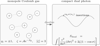
For the regulated dilute gas, $\partial\cdot B=2\pi q\delta$ pairs with $e^{+iq\sigma}$ using the Bianchi multiplier $-i\sigma\partial\cdot B/(2\pi)$. The leading compact-scalar action has the displayed kinetic coefficient and cosine. The positions are schematic; core interactions and higher harmonics are omitted, and $[\zeta]=3$.

The analogy with an ordinary electric plasma is literal. A test magnetic charge polarizes the monopole gas around it. The screening cloud cuts off the long-range magnetic Coulomb field. In the original gauge-field language, this means the photon is no longer massless. In the dual language, it means the dual photon is pinned by a periodic potential.

After powers of $v$ and $g_3^2$ from the determinant are restored, the useful semiclassical slogan is

$$m^2\sim (\text{microscopic mass})^2 e^{-\operatorname{const}\,v/g_3^2}.$$

This is the right physical scaling: the mass gap is nonanalytic at weak coupling. No finite order of perturbation theory can produce it.

Dual photon and sine-Gordon action

The dual formulation fixes the charged-insertion sign as well as the kinetic coefficient. First regulate the Gaussian functional integral and introduce a real local lift of $\sigma$ as the Fourier multiplier for the Bianchi constraint. On a topologically trivial region, with boundary terms controlled, the zero-monopole sector is

$$Z_0=\int \mathcal DB\,\mathcal D\sigma\, \exp\left[ -\int d^3x\,{B_\mu B_\mu\over2e^2} -{i\over2\pi}\int d^3x\,\sigma\,\partial_\mu B_\mu \right].$$

The local multiplier integration is over the real line: integrating a single angle only from zero to $2\pi$ would not impose a Dirac delta on an arbitrary real divergence. Flux-sector quantization and integer monopole vertices subsequently identify the dual scalar as compact, $\sigma\sim\sigma+2\pi$. On closed space its zero mode enforces total magnetic neutrality, and harmonic/flux sectors must also be included; the local Gaussian coefficient below is unchanged. On $\mathbb R^3$ one may instead allow flux through the large-distance boundary.

Integrating by parts makes the $B$ source $+i\partial_\mu\sigma/(2\pi)$. Complete the square:

$$-{B^2\over2e^2}+{i\over2\pi}B\cdot\partial\sigma =-{1\over2e^2}\left(B-{ie^2\over2\pi}\partial\sigma\right)^2 -{e^2\over8\pi^2}(\partial\sigma)^2.$$

The contour shift is valid in the finite positive Gaussian regulator. It gives the free dual action

$$S_{\rm dual,0}[\sigma] ={e^2\over8\pi^2}\int d^3x\,(\partial_\mu\sigma)^2.$$

A monopole of charge $q$ at $x_i$ changes the Bianchi identity by

$$\partial_\mu B_\mu(x)=2\pi q\delta^{(3)}(x-x_i).$$

Replace the constraint by $\partial\cdot B-2\pi q\delta_{x_i}=0$. Its multiplier is

$$-{i\over2\pi}\int\sigma\bigl(\partial\cdot B-2\pi q\delta_{x_i}\bigr) =-{i\over2\pi}\int\sigma\partial\cdot B+iq\sigma(x_i),$$

so the dual vertex is

$$e^{iq\sigma(x_i)}.$$

Summing independently over monopoles and anti-monopoles therefore gives

$$\sum_{N_+,N_-\ge0} {1\over N_+!N_-!} \left(\zeta\int d^3x\,e^{i\sigma(x)}\right)^{N_+} \left(\zeta\int d^3x\,e^{-i\sigma(x)}\right)^{N_-} = \exp\left[2\zeta\int d^3x\,\cos\sigma(x)\right].$$

Thus the regulated leading dilute monopole gas has the three-dimensional sine-Gordon description

$$\boxed{ S_{\rm dual}[\sigma] = \int d^3x\, \left[ {e^2\over8\pi^2}(\partial_\mu\sigma)^2 +2\zeta(1-\cos\sigma) \right]. }$$

The additive constant has been chosen so that the vacuum energy of the cosine term vanishes at $\sigma=0$.

As a check in the free dual Gaussian, $\langle\sigma(x)\sigma(y)\rangle=G(x-y)/K$ with $K=e^2/(4\pi^2)$. Its normal-ordered integer vertices give

$$\left\langle\prod_i:e^{iq_i\sigma(x_i)}:\right\rangle_0 =\exp\left[-{1\over2K}\sum_{i\ne j}q_iq_jG(x_i-x_j)\right],$$

which is precisely the Coulomb coefficient above, with the self-contractions assigned to the core fugacity. On a closed domain this statement also requires $\sum_iq_i=0$ from the zero mode. The plasma/dual-field method and magnetic-correlation interpretation are discussed in Polyakov 1987, § 4, pp. 65–68; the coefficients here follow the explicitly completed Gaussian in our unit-flux convention.

Expanding near a minimum,

$$2\zeta(1-\cos\sigma)=\zeta\sigma^2+O(\sigma^4),$$

so the dual photon has mass

$$\boxed{ m_\gamma^2={8\pi^2\zeta\over e^2} }$$

in this normalization. Since $\zeta=\mathcal A e^{-S_0}$,

$$m_\gamma^2={8\pi^2\mathcal A\over e^2}e^{-S_0}, \qquad m_\gamma\sim e^{-S_0/2}\times \text{power of microscopic scales}.$$

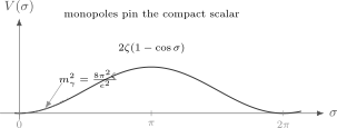
Monopoles generate a periodic potential for the compact dual photon $\sigma$. Expanding around any minimum gives a mass $m_\gamma$, which is nonperturbative in the microscopic coupling.

This mass is sometimes called a photon mass, but gauge invariance is not broken and the unbroken Abelian field receives no perturbative Proca term. The Gaussian saddle $B=ie^2\partial\sigma/(2\pi)$ is not a real off-shell operator identity. Differentiating the regulated $B$ Gaussian retains its contact term. At the quadratic dual-field level, the reduced momentum-space covariance is

$$\langle B_\mu(p)B_\nu(-p)\rangle_c =e^2\left(\delta_{\mu\nu}-{p_\mu p_\nu\over p^2+m_\gamma^2}\right).$$

As elsewhere, the momentum-conserving volume/delta factor is suppressed in this reduced covariance. At zero fugacity it is the transverse Maxwell covariance. For nonzero fugacity its nonlocal part has a massive pole; at separated points this gives

$$\langle B_\mu(x)B_\nu(0)\rangle_c\sim e^{-m_\gamma |x|}$$

up to powers of $|x|$. The mass gap is produced by magnetic instantons.

Wilson loops and the area law

The diagnostic for confinement is the Wilson loop

$$W(C)=\exp\left(i\oint_C a_\mu dx^\mu\right).$$

This is the charge-one Abelian component associated with a fundamental $SU(2)$ probe. The normalized fundamental trace at low energy combines it with its conjugate as $\cos\oint a$; charge reversal makes their leading large-loop expectations equal.

For a large rectangular loop of spatial size $R$ and Euclidean time size $T_E$,

$$\langle W(R,T_E)\rangle\sim e^{-V(R)T_E}.$$

If the loop obeys an area law,

$$\langle W(C)\rangle\sim e^{-T_{\rm string}\operatorname{Area}(C)},$$

then

$$V(R)=T_{\rm string}R$$

for large $R$. This is confinement: separating a pair of external electric charges costs energy proportional to their separation.

Let $\Sigma$ have the Stokes orientation $\partial\Sigma=C$, and define its surface distribution $\eta_\Sigma$ by $\int B\cdot\eta_\Sigma=\int_\Sigma B\cdot dS$. The insertion $W=\exp(i\int B\cdot\eta_\Sigma)$ adds this source to the same Gaussian. Its kinetic term becomes

$${K\over2}(\partial\sigma+2\pi\eta_\Sigma)^2,\qquad K={e^2\over4\pi^2}.$$

In a flat local patch with oriented normal coordinate $z$, $\eta_\Sigma=\widehat z\delta(z)$. Cancellation of the singular gradient requires

$$\Delta_{\widehat n}\sigma\equiv\sigma(0^+)-\sigma(0^-)=-2\pi, \qquad |\Delta_{\widehat n}\sigma|=2\pi.$$

This is a branch discontinuity of a compact field. Removing the cut by $\varphi=\sigma+2\pi H(z)$ gives the ordinary kinetic term and the same cosine, since $H$ is integer-valued away from the sheet. The continuous lift $\varphi$ connects neighboring values $0$ and $2\pi$ if the original branch tends to zero on both far sides.

Thus the magnitude of the winding is $2\pi$; reversing the loop reverses its oriented sign without changing the action. In the wall equations below we label this continuous neighboring-lift profile by $\sigma$. For a large loop, the leading saddle is a sine-Gordon wall on a minimal spanning surface. Its tension supplies the area term; perimeter and fluctuation corrections are not included in that leading expression. Inspect the boundary and normal orientations in the diagram.

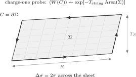
Schematic oriented spanning sheet, not a resolved wall profile. For $W=\exp(+i\oint a)$ the branch jump along the Stokes normal is $-2\pi$, with magnitude $2\pi$ as shown. Removing the branch cut yields the continuous neighboring-lift wall whose tension gives the leading area term for an unscreened unit probe. Charge-two strings can eventually break on heavy $W$ bosons.

For the charge-one probe in the normalization of this page, the exact numerical coefficient in $T_{\rm string}$ follows from the low-energy sine-Gordon action, while changes of charge convention rescale it. Its parametric form is

$$T_{\rm string}\sim e^2m_\gamma.$$

This is a useful formula to remember. The gauge coupling $e^2$ supplies the stiffness of the dual photon, and $m_\gamma$ supplies the inverse thickness of the wall. Their product has dimension two, as a string tension should in $2+1$ dimensions.

A useful normalization check is the exact sine-Gordon wall tension in this low-energy action. Write the kinetic term as

$${1\over2}K(\partial\sigma)^2, \qquad K={e^2\over4\pi^2},$$

and the potential as

$$V(\sigma)=2\zeta(1-\cos\sigma).$$

The static wall connecting neighboring vacua obeys the first-integral equation

$${1\over2}K(\sigma')^2=V(\sigma),$$

so its tension is

$$T_{\rm wall}=\int_0^{2\pi}d\sigma\,\sqrt{2K V(\sigma)} =8\sqrt{2K\zeta} =8K m_\gamma.$$

Thus, in this normalization,

$$T_{\rm wall}={2e^2\over\pi^2}m_\gamma.$$

The coefficient above is exact within this leading dilute-gas sine-Gordon action. Higher harmonics, determinant corrections, and a different normalization of the minimal electric probe change it. The relation $T\propto e^2m_\gamma$ is the robust semiclassical lesson.

Which electric charges remain confined?

The domain wall above describes the minimal charge-one Wilson loop. The ultraviolet completion also contains dynamical $W$ bosons of Abelian charge $2$. They can screen an external even charge: a charge-two string can break by producing a $W^+W^-$ pair once its energy is large enough. Parametrically, string breaking becomes favorable near

$$R_{\rm break}\sim {2m_W\over T_2},$$

where $T_2$ is the metastable charge-two string energy per length before breaking, not the unit-probe tension computed above. This estimate neglects binding energies and the detailed pair-creation process. An odd external charge cannot be completely screened by particles of charge $2$. It can only be shifted by an even amount and therefore retains the unit-charge string. Thus the asymptotic area law in this adjoint-only $SU(2)$ model applies to nontrivial $\mathbb Z_2$ center charge. Even-charge loops may display an intermediate area law but eventually cross over to string breaking and perimeter behavior.

This derivation also explains why simply giving a photon a mass is not the whole story. A massive noncompact photon would screen fields, but screening alone need not produce a Wilson-loop area law for electric charges. Compactness and the periodicity of the dual photon are essential: the Wilson loop is a topological defect for $\sigma$, and the defect must be filled by a domain wall.

Abelian confinement and the lesson for QCD

The three-dimensional model gives a controlled example of Abelian confinement. The low-energy gauge group is $U(1)$, and the asymptotically confined probes are the odd-charge, center-nontrivial external charges that cannot be screened by the massive $W$ bosons. The mechanism is magnetic disorder:

$$\text{monopole instanton gas} \quad\Longrightarrow\quad \text{dual-photon mass} \quad\Longrightarrow\quad \text{Wilson-loop area law}.$$

This is often called the Polyakov confinement mechanism.

In four Euclidean dimensions the same monopole solution is not localized in all spacetime directions. It traces out a worldline. A dilute collection of monopole loops would contribute schematically as

$$Z_{\rm loops}\sim \sum_{\text{closed loops }\Gamma} \exp[-M_{\rm mon}\operatorname{Length}(\Gamma)]\times(\text{fluctuation factors}).$$

In a regulated loop ensemble, the number of random closed loops can grow exponentially with length. This motivates a competition:

$$\text{action cost per unit length} \quad\text{versus}\quad \text{entropy per unit length}.$$

If the entropy gain exceeds the action cost, monopole loops proliferate. This is a heuristic magnetic-condensate picture behind the dual-superconductor analogy for confinement; unlike the three-dimensional dilute plasma, it is not a controlled derivation of confinement in ordinary four-dimensional Yang–Mills theory.

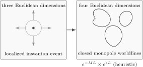
In three Euclidean dimensions a monopole is an instanton event. In four Euclidean dimensions it becomes a worldline. The displayed action–entropy competition is a heuristic loop-ensemble picture, not the controlled three-dimensional dilute-plasma derivation.

For non-Abelian QCD, the situation is subtler. There is no weakly coupled adjoint Higgs field in ordinary QCD that leaves a clean compact $U(1)$ theory with semiclassical monopoles. Perturbation theory explains asymptotic freedom, but not confinement by itself. Nonperturbatively, the expected infrared physics involves a mass gap and an area law for appropriate Wilson loops, but deriving this directly in continuum four-dimensional Yang–Mills theory remains much harder than in the three-dimensional Abelianized model.

The value of the three-dimensional model is conceptual and technical. It shows explicitly that topological defects can produce confinement in a weakly coupled calculation. It also teaches the right infrared variables: Wilson loops, compactness, magnetic disorder, dual fields, and defect condensation.

Example: Debye screening from the dual action

The sine-Gordon action immediately reproduces plasma screening. For small fluctuations around a vacuum, use

$$S_{\rm dual}\approx\int d^3x\, \left[ {e^2\over8\pi^2}(\partial\sigma)^2+ \zeta\sigma^2 \right].$$

The dual propagator is therefore

$$\langle \sigma(p)\sigma(-p)\rangle ={4\pi^2/e^2\over p^2+m_\gamma^2}, \qquad m_\gamma^2={8\pi^2\zeta\over e^2}.$$

A test magnetic charge couples as $e^{iq\sigma}$. At quadratic order, the interaction between two test magnetic charges is governed by the massive Green function

$$G_m(r)={e^{-m_\gamma r}\over4\pi r}.$$

Thus the monopole plasma converts the long-range Coulomb potential into a Yukawa potential. This is Debye screening. The same mass scale controls the thickness of the confining electric flux tube.

Summary

In three Euclidean dimensions, the monopole of a broken $SU(2)$ gauge theory is a finite-action instanton. The stated adjoint convention requires $\epsilon_{a\mu b}$ in its positive Higgs hedgehog. The Abelian map $a=-A^3/2$ then gives unit positive flux, fundamental charges $\pm1$, adjoint charges $\pm2$ and $e^2=g_3^2/4$ at tree level. With $m_\gamma\ll m_H,m_W$ and a regulated dilute core gas, the long-distance theory is compact $U(1)$ and its monopole events must be summed.

The dilute monopole gas is a Coulomb plasma. Dualizing the Abelian photon maps this plasma to a sine-Gordon theory for a compact scalar $\sigma$:

$$S_{\rm dual}=\int d^3x\, \left[ {e^2\over8\pi^2}(\partial\sigma)^2+2\zeta(1-\cos\sigma) \right].$$

The cosine term gives the dual photon a nonperturbative mass,

$$m_\gamma^2\propto {\zeta\over e^2} \propto {\mathcal A\over e^2}e^{-S_0},$$

and the Wilson loop becomes a domain-wall problem for the dual photon. The result is an area law,

$$\langle W(C)\rangle\sim e^{-T_{\rm string}\operatorname{Area}(C)}, \qquad T_{\rm string}\sim e^2m_\gamma.$$

This is confinement by monopole instantons in the declared regime. The first-order multiplier $-i\sigma\partial\cdot B/(2\pi)$ fixes both the positive-charge vertex and the oriented Wilson discontinuity; its magnitude determines the wall energy. Charge-two $W$ bosons screen even external charges, while odd center charge remains confined. The exactly massless-Higgs BPS limit and ordinary four-dimensional QCD require different infrared analyses.

Common pitfalls

Treating a three-dimensional monopole as a propagating particle. In three Euclidean dimensions it is an instanton event. In four Euclidean dimensions the analogous object is a worldline, and the physics becomes a question about loop proliferation.

Calling the dual-photon mass a perturbative Proca mass. Gauge invariance is unbroken; the mass gap arises from compactness and monopole events.

Using the BPS action as a photon-only effective theory. At zero scalar self-coupling the neutral Higgs is massless. The isolated monopole bound remains useful, but a theory retaining only the photon then omits a gapless mode.

Checking a charged sign only after summing to a cosine. Charge conjugation hides a reversed insertion in $\cos\sigma$. Check a fixed $q$ against the Bianchi constraint and retain the Gaussian contact term when computing magnetic correlators.

Equating a mass gap with electric confinement. Debye screening explains the dual mass, but the Wilson-loop area law follows because the loop forces a topological discontinuity of the compact dual scalar.

Ignoring screening by the heavy $W$ bosons. In fundamental-charge units the $W$ bosons have charge $2$. They can break even-charge strings, while an odd charge retains a nontrivial $\mathbb Z_2$ center charge and remains confined.

Promoting the four-dimensional analogy to a derivation. The controlled calculation is Abelianized and three-dimensional. Ordinary four-dimensional QCD has related magnetic-disorder ideas, but not the same weak-coupling derivation in flat space without additional structure.

Exercises

Exercise 1: Dimensions of the coupling and fugacity

Show by dimensional analysis that in three dimensions $[e^2]=1$ and $[\zeta]=3$, and check that

$$m_\gamma^2={8\pi^2\zeta\over e^2}$$

has the correct dimension.

Solution

The Maxwell action is

$$S={1\over4e^2}\int d^3x\,f_{\mu\nu}f_{\mu\nu}.$$

With the Wilson loop $\exp(i\oint a)$ dimensionless, $[a]+[x]=0$, so $[a]=1$ in mass units. Then $[f]=[\partial a]=2$, and $[f^2]=4$. Since $[d^3x]=-3$, the factor $1/e^2$ must have dimension $-1$, hence

$$[e^2]=1.$$

The fugacity $\zeta$ appears in the action as

$$\int d^3x\,\zeta\cos\sigma,$$

and $\sigma$ is dimensionless because it is compact. Therefore

$$[\zeta]=3.$$

Thus

$$\left[{\zeta\over e^2}\right]=3-1=2,$$

which is the dimension of a mass squared. The expression for $m_\gamma^2$ is dimensionally consistent.

Exercise 2: Dual-photon mass

Starting from

$$S_{\rm dual}[\sigma]=\int d^3x\, \left[ {e^2\over8\pi^2}(\partial\sigma)^2+2\zeta(1-\cos\sigma) \right],$$

derive the small-fluctuation mass of $\sigma$ around $\sigma=0$.

Solution

Expand the cosine:

$$1-\cos\sigma={\sigma^2\over2}+O(\sigma^4).$$

Then

$$2\zeta(1-\cos\sigma)=\zeta\sigma^2+O(\sigma^4).$$

The quadratic action is

$$S^{(2)}=\int d^3x\, \left[ {e^2\over8\pi^2}(\partial\sigma)^2+\zeta\sigma^2 \right].$$

Write it in the canonical quadratic form

$$S^{(2)}={1\over2}\int d^3x\, K\left[(\partial\sigma)^2+m_\gamma^2\sigma^2\right],$$

with

$$K={e^2\over4\pi^2}.$$

Matching the mass term gives

$${1\over2}Km_\gamma^2=\zeta,$$

so

$$m_\gamma^2={2\zeta\over K}={8\pi^2\zeta\over e^2}.$$

Exercise 3: Parametric string tension

Use the sine-Gordon action to estimate the parametric dependence of the Wilson-loop string tension. Explain why

$$T_{\rm string}\sim e^2m_\gamma.$$

Solution

A unit Wilson loop fixes a branch jump of magnitude $2\pi$. Removing that cut gives a continuous neighboring-lift domain wall transverse to the surface; its orientation does not change the energy.

The kinetic stiffness of the dual photon is

$$K={e^2\over4\pi^2},$$

because

$${e^2\over8\pi^2}(\partial\sigma)^2={1\over2}K(\partial\sigma)^2.$$

The wall thickness is set by the inverse dual-photon mass,

$$\ell_{\rm wall}\sim {1\over m_\gamma}.$$

Across the wall the field changes by an order-one amount, $\Delta\sigma=2\pi$, so the gradient is of order $m_\gamma$. The kinetic contribution per unit area is therefore

$$T_{\rm kin}\sim K(m_\gamma)^2\ell_{\rm wall} \sim K m_\gamma.$$

Since $K\sim e^2$, this gives

$$T_{\rm string}\sim e^2m_\gamma.$$

The potential contribution gives the same scaling by the equations of motion. Numerical factors depend on the normalization of the minimal Wilson loop and the precise sine-Gordon potential.

Exercise 4: Linear potential and string breaking

A large rectangular Wilson loop of spatial size $R$ and Euclidean time size $T_E$ satisfies

$$\langle W(R,T_E)\rangle\sim e^{-T_{\rm string}RT_E}.$$

Show that the corresponding static potential is linear. Then explain why a charge-two probe in the microscopic $SU(2)$ model does not remain confined at arbitrarily large separation, whereas a charge-one probe does.

Solution

The static potential is defined by the large-time behavior

$$\langle W(R,T_E)\rangle\sim e^{-V(R)T_E}$$

as $T_E\to\infty$. Comparing with the area-law form gives

$$V(R)T_E=T_{\rm string}RT_E,$$

so

$$V(R)=T_{\rm string}R.$$

Thus the energy required to separate external electric charges grows linearly with separation. This is confinement.

This last conclusion assumes that the external charge cannot be screened. In the normalization of this page, a dynamical $W$ boson has charge $2$. Pair creation can therefore screen a charge-two probe and break its string once

$$T_2R\gtrsim 2m_W.$$

Here $T_2$ is the pre-breaking charge-two string tension, with binding-energy corrections omitted from this threshold estimate. It is not the charge-one coefficient in the first part of the exercise. A charge-one probe cannot be neutralized by any number of charge-two $W$ bosons. It retains odd $\mathbb Z_2$ center charge and its string remains asymptotically stable in this adjoint-only model.

Exercise 5: Exact sine-Gordon wall tension

For the sine-Gordon action

$$S=\int d^3x\,\left[{1\over2}K(\partial\sigma)^2+2\zeta(1-\cos\sigma)\right],$$

compute the tension of a one-dimensional wall satisfying $\sigma(-\infty)=0$ and $\sigma(+\infty)=2\pi$. Express the answer in terms of $K$ and $m_\gamma^2=2\zeta/K$.

Solution

For a static wall depending on one coordinate $z$, the tension is

$$T=\int dz\,\left[{1\over2}K(\sigma')^2+V(\sigma)\right], \qquad V(\sigma)=2\zeta(1-\cos\sigma).$$

The equation of motion has the first integral

$${1\over2}K(\sigma')^2-V(\sigma)=0,$$

because both $\sigma'$ and $V$ vanish at $z=\pm\infty$. Therefore

$$T=\int dz\,2V(\sigma) =\int_0^{2\pi}d\sigma\,{2V(\sigma)\over\sigma'}.$$

Using

$$\sigma'=\sqrt{{2V(\sigma)\over K}},$$

gives

$$T=\int_0^{2\pi}d\sigma\,\sqrt{2K V(\sigma)}.$$

Since

$$V(\sigma)=4\zeta\sin^2{\sigma\over2},$$

we find

$$T=\sqrt{8K\zeta}\int_0^{2\pi}d\sigma\,\sin{\sigma\over2} =4\sqrt{8K\zeta}=8\sqrt{2K\zeta}.$$

Using $m_\gamma^2=2\zeta/K$ gives

$$T=8K m_\gamma.$$

For $K=e^2/(4\pi^2)$ this becomes $T=2e^2m_\gamma/\pi^2$ for the declared unit probe. Changing the probe charge changes the wall boundary condition; the charge-two breaking threshold must use its own pre-breaking energy.

References

• G. ’t Hooft, “Magnetic Monopoles in Unified Gauge Theories,” Nuclear Physics B 79 (1974), 276–284, doi:10.1016/0550-3213(74)90486-6. Open PDF, author copy.
• A. M. Polyakov, Gauge Fields and Strings, Contemporary Concepts in Physics, vol. 3, Harwood Academic Publishers, Chur, 1987, doi:10.1201/9780203755082.

Further reading

• T. Banks, R. Myerson, and J. Kogut, “Phase Transitions in Abelian Lattice Gauge Theories,” Nuclear Physics B 129 (1977), 493–510, doi:10.1016/0550-3213(77)90129-8.
• S. Coleman, Aspects of Symmetry: Selected Erice Lectures, Cambridge University Press, Cambridge, 1985, especially “The Magnetic Monopole Fifty Years Later.”
• A. M. Polyakov, “Compact Gauge Fields and the Infrared Catastrophe,” Physics Letters B 59 (1975), 82–84, doi:10.1016/0370-2693(75)90162-8.
• A. M. Polyakov, “Quark Confinement and Topology of Gauge Groups,” Nuclear Physics B 120 (1977), 429–458, doi:10.1016/0550-3213(77)90086-4.
• M. Srednicki, Quantum Field Theory, Cambridge University Press, Cambridge, 2007.
• J. Zinn-Justin, Quantum Field Theory and Critical Phenomena, 5th ed., Oxford University Press, Oxford, 2021.