Callan–Symanzik Scaling and Emergent Conformal Symmetry

The previous page treated scaling dimensions as the language of critical correlators. This page explains how that language arises dynamically. Near a continuous phase transition, perturbation theory first produces logarithms such as $\log(\Lambda/k)$: the same fluctuation physics is being sampled over many length scales. The renormalization group reorganizes those logarithms into scaling laws.

The central object is the critical two-point function of the order-parameter field. For the undifferentiated massless Gaussian scalar in $d>2$,

$$G_0(k)={1\over k^2}, \qquad G_0(x)\sim {1\over |x|^{d-2}},$$

so the engineering dimension of a scalar field is $(d-2)/2$. At an interacting fixed point this becomes

$$G(k)\sim {1\over k^{2-\eta}}, \qquad G(x)\sim {1\over |x|^{d-2+\eta}}, \qquad \Delta_\phi={d-2+\eta\over2}.$$

The exponent $\eta$ is twice the anomalous part of the field dimension. The Callan–Symanzik equation gives the differential statement behind this result. At the upper critical dimension, a marginally irrelevant coupling instead produces operator-dependent logarithmic corrections. Conformal symmetry requires an additional condition on the stress tensor.

Required background. Lesson 12 supplies the scaling-field and critical-exponent dictionary used throughout this page.

Helpful background. Lesson 4 introduces the upper critical dimension, while Lesson 5 develops the Wilson–Fisher fixed point and anomalous dimensions perturbatively.

Engineering dimension and the Gaussian propagator

Renormalization convention

We work in Euclidean $d$ dimensions. The scalar field theory used as the standard example is

$$S=\int d^d x\,\left[{1\over2}(\partial\phi)^2+{1\over2}r\phi^2+{\mu^\epsilon g\over4!}\phi^4\right], \qquad \epsilon=4-d.$$

Counterterms are understood, and the parameter $r$ is tuned to its critical value. The renormalized coupling $g$ is dimensionless; the coefficient $u=\mu^\epsilon g$ has mass dimension $\epsilon$. Strip the momentum-conserving delta function from the propagator:

$$\langle\phi(k)\phi(k')\rangle_c=(2\pi)^d\delta^{(d)}(k+k')G(k), \qquad \Gamma^{(2)}(k)=G(k)^{-1}.$$

For a renormalized field $\phi_R$, we use

$$\phi_0=Z_\phi^{1/2}\phi_R, \qquad \gamma_\phi(g)={1\over2}\mu{\partial\over\partial\mu}\log Z_\phi\bigg|_{\rm bare}, \qquad \beta(g)=\mu{\partial g\over\partial\mu}\bigg|_{\rm bare}.$$

With this convention, the fixed-point dimension is

$$\Delta_\phi={d-2\over2}+\gamma_\phi(g_*), \qquad \eta=2\gamma_\phi(g_*).$$

The operator anomalous dimensions below use the same convention: $\Delta_O=\Delta_O^{(0)}+\gamma_O(g_*)$ for a multiplicatively renormalized scaling operator.

The free massless scalar action is

$$S_0={1\over2}\int d^d x\,(\partial\phi)^2.$$

Under a dilation $x\mapsto \lambda x$, the kinetic term remains invariant if

$$\phi(x)\mapsto \lambda^{\Delta_\phi^{(0)}}\phi(\lambda x), \qquad \Delta_\phi^{(0)}={d-2\over2}.$$

Equivalently, the free propagator satisfies

$$G_0(\lambda x)=\lambda^{-(d-2)}G_0(x).$$

The explicit Fourier transform is

$$G_0(x)=\int {d^d k\over(2\pi)^d}\,{e^{ik\cdot x}\over k^2} ={\Gamma(d/2-1)\over4\pi^{d/2}}{1\over |x|^{d-2}} \qquad (d>2).$$

Thus

$$G_0(x)\sim {1\over |x|^{2\Delta_\phi^{(0)}}}.$$

At this level, scaling is just dimensional analysis. The lesson of critical phenomena is that the true long-distance field can scale with a dimension different from its engineering dimension.

Logarithms before powers

Interactions first appear perturbatively as corrections to the inverse propagator and to the interaction vertex. Write the exact inverse propagator schematically as

$$G^{-1}(k)=k^2+r+\Sigma(k),$$

where $\Sigma(k)$ is the self-energy. At criticality the mass-like term is tuned so that

$$G^{-1}(0)=0.$$

The remaining momentum dependence can contain logarithms. In four dimensions, $g\phi^4$ is classically marginal, and typical loop integrals behave like

$$\int_k^\Lambda {d^4p\over p^4} \sim \log {\Lambda\over k}.$$

Therefore a critical inverse propagator can have the schematic form

$$G^{-1}(k)=k^2\left[1+A g^2\log {\Lambda\over k}+\cdots\right].$$

The exact power of $g$ depends on the quantity being studied. In ordinary $\phi^4$ theory the field anomalous dimension begins at two loops; the energy operator $\phi^2$ already receives an anomalous dimension at one loop. The structural point is the same: when $k\ll\Lambda$, the logarithm becomes large and fixed-order perturbation theory is not the right expansion.

The same issue appears in the four-point vertex. In $d=4$ one finds, schematically,

$$\Gamma_4(k)=g-Bg^2\log {\Lambda\over k}+\cdots.$$

The logarithm says that the coupling measured at scale $k$ is not the same as the coupling defined at the cutoff. Physics at different scales is being compared.

The upper critical dimension and logarithmic scaling

The engineering dimensions of the quartic coefficient and its dimensionless counterpart are

$$[u]=4-d,\qquad [g]=0,\qquad u=\mu^{4-d}g.$$

Thus $d=4$ is the upper critical dimension of the Ising universality class. Above four dimensions the quartic interaction is irrelevant and mean-field exponents are correct. Below four dimensions the interaction flows to the Wilson–Fisher fixed point. Exactly at four dimensions it is marginally irrelevant in the infrared, so powers acquire logarithmic corrections.

Near $d=4$, the beta function has the form

$$\beta(g)=\mu {dg\over d\mu}=-\epsilon g+b g^2+O(g^3), \qquad b>0.$$

For $d=4-\epsilon$, there is an interacting fixed point

$$g_*={\epsilon\over b}+O(\epsilon^2).$$

At this fixed point, separated-point critical correlators of scaling operators are powers. At exactly $d=4$, take a weak positive initial coupling $g_0$ at $\mu_0=a^{-1}$. In infrared time $L=\log(\mu_0/\mu)$, the leading beta function gives

$${dg\over dL}=-b g^2, \qquad g(L)={g_0\over1+b g_0L}.$$

Thus $g(L)\sim1/(bL)$ for $b g_0L\gg1$. This is the controlled infrared branch; a negative initial coupling is not covered. Whether a correlator gains a power of a logarithm depends on its anomalous dimension, which the Callan–Symanzik equation integrates.

The Callan–Symanzik equation

Let

$$G_R^{(n)}(x_1,\ldots,x_n;g,\mu) =\langle \phi_R(x_1)\cdots\phi_R(x_n)\rangle_c$$

be a renormalized critical correlator. The auxiliary scale $\mu$ is introduced by renormalization. Bare quantities do not depend on $\mu$, so changing $\mu$ must be compensated by changing the renormalized coupling and the normalization of the fields. This gives the Callan–Symanzik equation

$$\boxed{ \left[\mu {\partial\over\partial\mu} +\beta(g){\partial\over\partial g} +n\gamma_\phi(g)\right]G_R^{(n)}=0. }$$

For a product of multiplicatively renormalized operators $O_i$, the last term becomes $\sum_i\gamma_{O_i}(g)$. If operators with the same quantum numbers mix, the anomalous dimensions form a matrix and the equation acts on the corresponding vector of correlators.

The equation is best read by the method of characteristics. Define the running coupling by

$${d\bar g(\ell)\over d\ell}=\beta(\bar g(\ell)), \qquad \bar g(0)=g,$$

where increasing $\ell$ corresponds to changing the reference scale $\mu\mapsto e^\ell\mu$. Then

$$G_R^{(n)}(x_i;g,\mu) = \exp\left[+n\int_0^\ell d\ell'\,\gamma_\phi(\bar g(\ell'))\right] G_R^{(n)}(x_i;\bar g(\ell),e^\ell\mu).$$

The plus sign follows directly from transporting the correlator from the endpoint of the characteristic back to its starting point. Equivalently,

$$G_R^{(n)}(x_i;\bar g(\ell),e^\ell\mu) = \exp\left[-n\int_0^\ell d\ell'\,\gamma_\phi(\bar g(\ell'))\right] G_R^{(n)}(x_i;g,\mu).$$

These expressions transport the reference scale at fixed coordinates; they are not yet physical-distance scaling laws. In infrared time $L=-\ell$, $d\bar g/dL=-\beta(\bar g)$. The figure illustrates an approach to a fixed point with this sign convention.

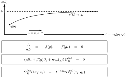
The quantitative illustration solves $dg/dL=-\omega(g-g_*)$ with $g_*=1$, $g_0=0.2$ and $\omega=0.5$ over $0\leq L\leq8$: $g(L)=g_*+(g_0-g_*)e^{-\omega L}$. It is an illustrative linearized flow, not a fitted beta function. The initial point is at $L=0$; $\mu=\mu_0e^{-L}$ decreases to the right.

At a fixed point,

$$\beta(g_*)=0, \qquad \gamma_\phi(g_*)=\gamma_\phi^*.$$

Combining the Callan–Symanzik equation with ordinary dimensional analysis gives

$$G_R^{(n)}(\lambda x_1,\ldots,\lambda x_n) =\lambda^{-n\Delta_\phi}G_R^{(n)}(x_1,\ldots,x_n),$$

where

$$\boxed{ \Delta_\phi={d-2\over2}+\gamma_\phi^*. }$$

For the two-point function,

$$G(x)=\langle\phi(x)\phi(0)\rangle_c \sim {1\over |x|^{2\Delta_\phi}} ={1\over |x|^{d-2+\eta}},$$

with

$$\boxed{\eta=2\gamma_\phi^*.}$$

Momentum space gives the equivalent form

$$\boxed{ G(k)\sim {1\over k^{2-\eta}}, \qquad G^{-1}(k)\sim k^{2-\eta}. }$$

This is the cleanest interpretation of the anomalous exponent: it is the fixed-point value of the field-renormalization part of the RG flow.

Operator-dependent logarithms in four dimensions

To compare physical separations $R=|x|=ae^L$ at a fixed reference normalization, combine the characteristic solution with engineering scaling. For an operator of engineering dimension $\Delta_O^{(0)}$, the separated two-point function has the RG-improved form

$$\begin{aligned} \langle O(x)O(0)\rangle_c &=R^{-2\Delta_O^{(0)}}A_O(L)\,\mathcal M_O(g(L)),\\ A_O(L)&=\exp\left[-2\int_0^L\gamma_O(g(s))\,ds\right]. \end{aligned}$$

Here $\mathcal M_O$ is the matching amplitude at a reference separation of order the running cutoff; assume it has a finite nonzero Gaussian limit. Contact terms are excluded. The minus sign belongs to this physical-distance comparison. Forward transport of the reference scale at fixed coordinates instead gives $d\log G_R^{(2)}/dL=+2\gamma_O$: the two operations must not be interchanged.

For the elementary scalar, $\gamma_\phi=c_\phi g^2+O(g^3)$, whereas the energy operator has $\gamma_\epsilon=c_\epsilon g+O(g^2)$. Inserting the leading running coupling and retaining the displayed anomalous dimensions gives

$$\begin{aligned} A_\phi(L)&=\exp\left[-{2c_\phi g_0\over b} \left(1-{1\over1+b g_0L}\right)\right],\\ A_\epsilon(L)&=(1+b g_0L)^{-2c_\epsilon/b}. \end{aligned}$$

The elementary field factor approaches a finite constant, with inverse-logarithmic corrections. It has no nonzero leading power of $\log R$. The energy factor does have such a power. Higher orders change matching constants and subleading corrections; this contrast follows from integrating $g^2$ versus $g$. The perturbative orders and finite elementary-field renormalization are given in Zinn-Justin 2021, §17.2, pp. 423–424, Eqs. 17.14–17.16.

The Ising specific-heat logarithm

For the one-component scalar, $c_\epsilon/b=1/3$. The source uses $\eta=2\gamma_\phi$ and $\eta_2=-\gamma_\epsilon$; these translations fix the signs here. With $\Delta_\epsilon^{(0)}=2$, the critical energy correlation in the scaling window is therefore proportional to

$$\langle\epsilon(x)\epsilon(0)\rangle_c \sim R^{-4}(1+b g_0\log(R/a))^{-2/3}.$$

As in Lesson 12, the thermal response integrates this connected correlator. In four dimensions the radial measure contributes $R^3dR$, so the singular window contribution is, up to angular and matching factors,

$$\begin{aligned} C_{\rm window}&\propto\int_0^{L_\xi} {dL\over(1+b g_0L)^{2/3}}\\ &={3\over b g_0}\left[(1+b g_0L_\xi)^{1/3}-1\right], \qquad L_\xi=\log(\xi/a). \end{aligned}$$

Let $\hat\tau_0=a^2\tau$ be the dimensionless initial thermal scaling coupling to the renormalized energy operator. Its normalization is specific to this four-dimensional theory; no signed two-dimensional Majorana mass convention is implied. The leading thermal flow and its stopping condition are

$$\begin{aligned} {d\log|\hat\tau|\over dL}&=2-c_\epsilon g(L),\\ |\hat\tau(L_\xi)|&\sim1,\\ 2L_\xi-\tfrac13\log(1+b g_0L_\xi)&\simeq \log{1\over|\hat\tau_0|}. \end{aligned}$$

Thus $L_\xi=\tfrac12\log(1/|\hat\tau_0|)$ to leading logarithmic order. Substitution gives

$$C_{\rm sing}\sim\left[\log{1\over|\hat\tau_0|}\right]^{1/3}.$$

Physical heat capacity also includes a regular background, the temperature-to-source conversion and nonuniversal matching amplitudes. This argument fixes the leading logarithmic exponent, not an exact thermodynamic function. The additive renormalization of the response and the general exponent $(4-N)/(N+8)$ appear in Zinn-Justin 2021, §17.2, p. 425, Eqs. 17.23–17.27.

The figure isolates the slow running and the integrated energy response in dimensionless variables.

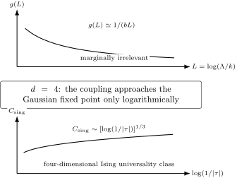
The plotted functions are $g/g_0=1/(1+s)$ and $H(s)=3[(1+s)^{1/3}-1]$ for $0\leq s\leq30$, with $s=b g_0L$. The second is the normalized integral of $(1+s)^{-2/3}$; it illustrates the scaling-window response, not an exact heat-capacity curve. These are quantitative plots of the stated leading-flow functions.

Skeleton equations and self-consistent scaling

There is another way to think about anomalous exponents. Instead of computing a few diagrams with bare propagators, write self-consistent equations for dressed quantities. The exact two-point function satisfies a Dyson equation

$$G^{-1}(k)=G_0^{-1}(k)+\Sigma(k),$$

where $\Sigma$ is the self-energy. A schematic four-point relation can be written

$$\Gamma_4=u+\Phi[G,\Gamma_4,\Gamma_6,\ldots],$$

where $\Phi$ stands for the appropriate dressed kernels, higher vertices and counterterms. This notation is not a closed exact equation for $G$ and $\Gamma_4$ alone. Any truncation must specify which kernels are retained and how it is renormalized.

At a fixed point, the only scale is momentum itself. It is therefore natural to try

$$G(k)\sim {1\over |k|^{2-\eta}}.$$

The four-point vertex has its own scaling. With the overall momentum-conserving delta function stripped off, its fixed-point momentum homogeneity degree is

$$d-4\Delta_\phi =d-2(d-2+\eta) =4-d-2\eta.$$

This is distinct from its engineering mass dimension $\epsilon=4-d$ at fixed renormalized-field convention. For nonexceptional external momenta scaled together by a characteristic magnitude $k$, a dimensionally consistent representative is

$$\Gamma_4(k;\mu)\sim \mu^{2\eta}k^{\epsilon-2\eta} \,\mathcal F(\text{momentum ratios}).$$

Homogeneity is a necessary consistency check on the complete equation. It does not determine $\eta$ without the dynamics of its kernels, nor validate an unspecified truncation.

Relevant perturbations and scaling forms

A critical point is a fixed point only after relevant perturbations have been tuned. For the Ising class the two most important perturbations are the temperature-like coupling and the magnetic field:

$$S=S_*+\tau\int d^d x\,\epsilon(x)-h\int d^d x\,\sigma(x)+\cdots.$$

The physical sources have mass dimensions $y_t$ and $y_h$. Define initial dimensionless scaling couplings $\hat\tau=a^{y_t}\tau$ and $\hat h=a^{y_h}h$. Near a fixed point their growth under blocking uses infrared time $L$, not the ultraviolet time $\ell$:

$${d\hat\tau\over dL}=y_t\hat\tau+\cdots, \qquad {d\hat h\over dL}=y_h\hat h+\cdots,$$

where

$$y_t=d-\Delta_\epsilon, \qquad y_h=d-\Delta_\sigma.$$

Solving the corresponding Callan–Symanzik equation gives the scaling form

$$\langle O(x)O(0)\rangle_\tau ={1\over |x|^{2\Delta_O}} \Phi_O\left(\tau |x|^{y_t}\right).$$

The correlation length is the value of $|x|$ at which the scaling variable becomes order one:

$$|\tau| \xi^{y_t}\sim1, \qquad {\xi\over a}\sim |\hat\tau|^{-1/y_t}.$$

Therefore

$$\nu={1\over y_t}={1\over d-\Delta_\epsilon},$$

which matches the scaling-dimension dictionary from the previous page. This fixed-point power law assumes no additional marginal running; the four-dimensional stopping equation above shows how logarithms modify it. In ultraviolet time $\ell=-L$, the linearized eigenvalues have the opposite sign.

Emergent scale invariance

A continuum critical point is obtained by taking a limit in which the microscopic lattice spacing $a$ becomes invisible compared with the physical correlation length:

$$a\ll |x|\ll \xi.$$

Exactly at criticality, $\xi=\infty$, and the long-distance theory has no intrinsic scale. This is emergent scale invariance. It does not mean the microscopic lattice was scale invariant. It means the RG flow has forgotten most microscopic details and landed on a fixed point.

The phrase “fixed point” should be taken literally. Under coarse graining and rescaling, the effective action returns to itself, up to field normalization and irrelevant corrections:

$$S_*[\phi]\mapsto S_*[\phi]+\text{redundant changes}.$$

Correlation functions then obey homogeneous scaling laws. For a scalar scaling operator,

$$\langle O(\lambda x_1)\cdots O(\lambda x_n)\rangle = \lambda^{-n\Delta_O} \langle O(x_1)\cdots O(x_n)\rangle.$$

Scale invariance alone does not yet give the full conformal transformation law. The next step is to understand when a scale-invariant local theory also has invariance under transformations that rescale distances by a position-dependent factor.

First hint of conformal symmetry

Consider an infinitesimal coordinate transformation in flat Euclidean space,

$$x^\mu\mapsto x'^\mu=x^\mu+\xi^\mu(x).$$

The flat metric changes according to

$$ds'^2 =\delta_{\mu\nu}\,dx'^\mu dx'^\nu =\left(\delta_{\rho\sigma} +\partial_\rho\xi_\sigma +\partial_\sigma\xi_\rho\right)dx^\rho dx^\sigma +O(\xi^2).$$

The transformation is conformal if it preserves angles, equivalently if the metric changes only by a local scale factor:

$$ds'^2=\rho(x)\,ds^2.$$

To first order this means

$$\partial_\rho\xi_\sigma+ \partial_\sigma\xi_\rho=2\lambda(x)\delta_{\rho\sigma}.$$

Taking the trace gives

$$2\partial\cdot\xi=2d\lambda(x),$$

so

$$\boxed{ \partial_\mu\xi_\nu+ \partial_\nu\xi_\mu ={2\over d}(\partial\cdot\xi)\delta_{\mu\nu}. }$$

This is the conformal Killing equation. Translations and rotations solve it with $\partial\cdot\xi=0$; dilations solve it with $\xi^\mu=cx^\mu$; special conformal transformations give the remaining solutions in $d>2$.

The following map makes local angle preservation visible: compare the tangent vectors, whose lengths are rescaled by the same factor.

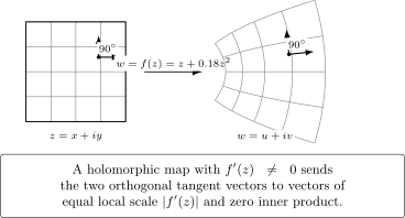
The quantitative grids use $f(z)=z+0.18z^2$ on $-1.2\leq\operatorname{Re}z,\operatorname{Im}z\leq1.2$, where $f'(z)\neq0$. At $P=0.55+0.35i$, the two perpendicular input vectors have length $0.52$; their displayed images are the derivative images under $f'(P)=1.198+0.126i$, not finite chords of the nonlinear map. Both panels use the same coordinate scale. The image vectors remain perpendicular and have equal length.

The connection to RG is through the stress tensor. Assume a local symmetric conserved stress tensor and a local conserved dilation current of the form

$$D_\mu=x^\nu T_{\mu\nu}-V_\mu,$$

where $V_\mu$ is a possible virial current. Conservation gives

$$T^\mu_{\ \mu}=\partial^\mu V_\mu.$$

If the virial current is absent, or if it can be removed by improving the stress tensor, then

$$T^\mu_{\ \mu}=0.$$

Write the improved symmetric conserved tensor as $T'$. Its special-conformal currents are

$$\begin{aligned} K^\mu_{(\alpha)}&=(2x_\alpha x_\nu-x^2\delta_{\alpha\nu})T'^{\mu\nu},\\ \partial_\mu K^\mu_{(\alpha)}&=2x_\alpha T'^\mu{}_{\mu}=0. \end{aligned}$$

Differentiation gives the last equality using both symmetry and conservation; tracelessness alone would not suffice. Whether such an improvement exists is the substantive condition. The virial criterion and improvement are discussed in Nakayama 2014, arXiv v4, §2.3, Eqs. 2.22–2.31.

In two dimensions, a sufficient enhancement theorem assumes unitarity, Poincaré invariance with causality, a discrete scaling spectrum, a local conserved dilation current, and an unbroken scale-invariant vacuum, with a well-defined local stress tensor. Its proof combines stress-tensor conservation with positivity to force the trace to vanish. See Nakayama 2014, arXiv v4, §5.1. This theorem does not establish an unconditional implication in arbitrary dimension. Scale versus conformal invariance develops the hypotheses and possible obstructions.

In two dimensions, the conformal Killing equation becomes especially strong. Writing

$$z=x+iy, \qquad \xi(z)=\xi^1(x,y)+i\xi^2(x,y),$$

one obtains

$$\partial_x\xi^1=\partial_y\xi^2, \qquad \partial_x\xi^2=-\partial_y\xi^1.$$

These are the Cauchy–Riemann equations,

$$\partial_{\bar z}\xi(z)=0.$$

Thus two-dimensional infinitesimal conformal transformations are locally holomorphic functions. This is the first glimpse of the infinite-dimensional symmetry that will dominate the CFT part of the course.

Example: fixed-point solution of the two-point equation

Take the critical two-point function in momentum space. Dimensional analysis says that before anomalous scaling is included, the propagator has momentum dimension $-2$:

$$G_R(k;g_*,\mu)=\mu^{-2}F(k/\mu).$$

At the fixed point, the Callan–Symanzik equation is

$$\left[\mu {\partial\over\partial\mu}+2\gamma_\phi^*\right]G_R(k;g_*,\mu)=0.$$

Since $G_R$ depends on $\mu$ through $k/\mu$ and through the engineering prefactor,

$$\mu {\partial G_R\over\partial\mu} =-2G_R-k{\partial G_R\over\partial k}.$$

The fixed-point equation becomes

$$-k{\partial G_R\over\partial k}-2G_R+2\gamma_\phi^*G_R=0.$$

Hence

$$k{\partial G_R\over\partial k}=(-2+2\gamma_\phi^*)G_R.$$

Solving gives

$$G_R(k)\propto k^{-2+2\gamma_\phi^*}.$$

Using $\eta=2\gamma_\phi^*$,

$$\boxed{G_R(k)\propto {1\over k^{2-\eta}}.}$$

Fourier transformation gives

$$G_R(x)\propto {1\over |x|^{d-2+\eta}}.$$

The anomalous exponent is therefore not an independent assumption; it is the fixed-point value of the RG field-renormalization function.

Summary

Perturbation theory near a critical point produces logarithms such as $\log(\Lambda/k)$. These logarithms are warnings that the same physics is being compared at several scales. The Callan–Symanzik equation turns that warning into a tool: it tracks how couplings and operator normalizations change with the renormalization scale.

At an RG fixed point,

$$\beta(g_*)=0,$$

and the Callan–Symanzik equation becomes a scaling equation. The field dimension becomes

$$\Delta_\phi={d-2\over2}+\gamma_\phi^*,$$

and the critical propagator behaves as

$$G(k)\sim {1\over k^{2-\eta}}, \qquad G(x)\sim {1\over |x|^{d-2+\eta}}.$$

Relevant physical sources produce dimensionless variables such as $\tau |x|^{y_t}$ and $\xi/a\sim|\hat\tau|^{-1/y_t}$. At the upper critical dimension, the elementary field has finite RG normalization with inverse-log corrections, while the energy operator’s normalization generates the Ising specific-heat logarithm with exponent $1/3$.

Finally, a local fixed point often does more than scale. If the stress tensor can be improved to be traceless, scale symmetry extends to conformal symmetry. Infinitesimally, conformal transformations are the solutions of

$$\partial_\mu\xi_\nu+ \partial_\nu\xi_\mu={2\over d}(\partial\cdot\xi)\delta_{\mu\nu}.$$

The next page studies these transformations directly.

Common pitfalls

A logarithm in perturbation theory is not itself an anomalous dimension. The anomalous dimension is obtained after RG improvement, and at a true fixed point it becomes a number.

The cutoff factor in expressions such as $G^{-1}(k)\sim \Lambda^\eta k^{2-\eta}$ is not universal. It reflects the normalization of the microscopic field. The exponent of $k$ is the universal part.

The upper critical dimension is special. A marginally irrelevant interaction does not give every operator a nonzero leading logarithmic power. Integrate that operator’s anomalous dimension, including its first nonvanishing order in $g$.

The self-energy $\Sigma(k)$ must be interpreted after mass tuning. A constant term in $\Sigma(0)$ shifts the critical temperature; the anomalous critical propagator comes from the nonanalytic momentum dependence at the tuned point.

Scale invariance and conformal invariance are not identical statements. The bridge between them involves locality, the stress tensor, and the possibility of improving the trace.

Exercises

Exercise 1: Gaussian field dimension

Derive the engineering dimension of a free scalar field in $d$ Euclidean dimensions from

$$S_0={1\over2}\int d^d x\,(\partial\phi)^2.$$

For $d>2$, show that the separated-point Gaussian two-point function behaves as $G_0(x)\sim |x|^{-(d-2)}$.

Solution

Under $x\mapsto \lambda x$, the measure scales as

$$d^d x\mapsto \lambda^{-d}d^d x$$

if we rewrite the transformed action in terms of the original coordinate. The derivative scales as

$$\partial\mapsto \lambda\partial.$$

Let

$$\phi(x)\mapsto \lambda^\Delta\phi(\lambda x).$$

Then the kinetic term scales as

$$\int d^d x\,(\partial\phi)^2 \mapsto \lambda^{-d}\lambda^{2+2\Delta} \int d^d x\,(\partial\phi)^2.$$

Scale invariance requires

$$-d+2+2\Delta=0,$$

so

$$\Delta={d-2\over2}.$$

For $d>2$, the massless scalar covariance has no infrared obstruction at nonzero separation and its exponent is twice the scaling dimension:

$$G_0(x)=\langle\phi(x)\phi(0)\rangle\sim {1\over |x|^{2\Delta}} ={1\over |x|^{d-2}}.$$

Exercise 2: Fixed-point propagator from Callan–Symanzik

Assume the fixed-point Callan–Symanzik equation for the critical two-point function is

$$\left[\mu {\partial\over\partial\mu}+2\gamma_\phi^*\right]G_R(k;\mu)=0,$$

and that dimensional analysis gives $G_R(k;\mu)=\mu^{-2}F(k/\mu)$. Show that

$$G_R(k)\propto k^{-2+\eta}, \qquad \eta=2\gamma_\phi^*.$$

Solution

Since

$$G_R(k;\mu)=\mu^{-2}F(k/\mu),$$

we have

$$\mu{\partial G_R\over\partial\mu} =-2G_R-k{\partial G_R\over\partial k}.$$

Substitute this into the fixed-point Callan–Symanzik equation:

$$-k{\partial G_R\over\partial k}-2G_R+2\gamma_\phi^*G_R=0.$$

Thus

$$k{\partial G_R\over\partial k}=(-2+2\gamma_\phi^*)G_R.$$

Solving,

$$G_R(k)=Ck^{-2+2\gamma_\phi^*}.$$

With $\eta=2\gamma_\phi^*$,

$$G_R(k)=Ck^{-2+\eta}={C\over k^{2-\eta}}.$$

Exercise 3: Multiplicative logarithms from a marginal coupling

Let $L=\log(|x|/a)$ be infrared RG time. Suppose a marginally irrelevant coupling obeys

$${dg\over dL}=-b g^2, \qquad b>0,$$

Take $g(0)=g_0>0$ in the weak-coupling regime. Let a multiplicatively renormalized composite operator have $\gamma_O(g)=c g+O(g^2)$ in this page’s convention and a finite nonzero Gaussian matching amplitude. Show that its separated connected two-point function receives a leading logarithmic correction of the form

$$\langle O(x)O(0)\rangle_c \sim {1\over |x|^{2\Delta_O^{(0)}}} \left(\log {|x|\over a}\right)^{-2c/b},$$

for $b g_0\log(|x|/a)\gg1$, up to a constant amplitude and subleading logarithms.

Solution

The leading running coupling is $g(L)=g_0/(1+b g_0L)$. Integrating from the finite initial scale avoids using the large-$L$ approximation at $L=0$:

$$\int_0^L c g(s)\,ds={c\over b}\log(1+b g_0L).$$

The physical-distance normalization factor is consequently

$$A_O(L)=\exp\left[-2\int_0^L c g(s)\,ds\right] =(1+b g_0L)^{-2c/b}\sim \text{const.}\,L^{-2c/b}.$$

Since $L=\log(|x|/a)$ for a separation $|x|$, the correlator becomes

$$\langle O(x)O(0)\rangle_c \sim {1\over |x|^{2\Delta_O^{(0)}}} \left(\log {|x|\over a}\right)^{-2c/b}.$$

The displayed negative exponent follows from the declared dimension convention. Higher-order anomalous dimensions and the matching amplitude supply subleading terms without changing this leading power.

Exercise 4: Derive the conformal Killing equation

Starting from

$$x'^\mu=x^\mu+\xi^\mu(x),$$

show that angle preservation to first order requires

$$\partial_\mu\xi_\nu+ \partial_\nu\xi_\mu ={2\over d}(\partial\cdot\xi)\delta_{\mu\nu}.$$

Solution

The transformed differential is

$$dx'^\mu=dx^\mu+\partial_\rho\xi^\mu dx^\rho.$$

Thus

$$ds'^2=\delta_{\mu\nu}dx'^\mu dx'^\nu =\left(\delta_{\rho\sigma} +\partial_\rho\xi_\sigma +\partial_\sigma\xi_\rho\right)dx^\rho dx^\sigma +O(\xi^2).$$

A conformal transformation preserves angles, so it may only multiply the metric by a scalar function:

$$ds'^2=(1+2\lambda(x))\delta_{\rho\sigma}dx^\rho dx^\sigma.$$

Equating coefficients gives

$$\partial_\rho\xi_\sigma+ \partial_\sigma\xi_\rho=2\lambda(x)\delta_{\rho\sigma}.$$

Taking the trace yields

$$2\partial\cdot\xi=2d\lambda,$$

so

$$\lambda={1\over d}\partial\cdot\xi.$$

Substituting back gives

$$\partial_\mu\xi_\nu+ \partial_\nu\xi_\mu ={2\over d}(\partial\cdot\xi)\delta_{\mu\nu}.$$

Exercise 5: Cauchy–Riemann form in two dimensions

In two Euclidean dimensions, set

$$\xi(z)=\xi^1(x,y)+i\xi^2(x,y), \qquad z=x+iy.$$

Show that the conformal Killing equation is equivalent to $\partial_{\bar z}\xi=0$.

Solution

For $d=2$, the conformal Killing equation is

$$\partial_i\xi_j+ \partial_j\xi_i=(\partial_k\xi_k)\delta_{ij}.$$

The $11$ component gives

$$2\partial_x\xi^1=\partial_x\xi^1+\partial_y\xi^2,$$

so

$$\partial_x\xi^1=\partial_y\xi^2.$$

The $12$ component gives

$$\partial_x\xi^2+\partial_y\xi^1=0.$$

These are precisely the Cauchy–Riemann equations for $\xi^1+i\xi^2$. Therefore

$$\partial_{\bar z}\xi=0.$$

References

• Nakayama, Yu. “Scale invariance vs conformal invariance.” arXiv:1302.0884v4 (28 February 2014). Versioned HTML. The section and equation locators above refer to this version.
• Zinn-Justin, Jean. Quantum Field Theory and Critical Phenomena. 5th ed. Oxford University Press, 2021. DOI.

Further reading

• Callan, Curtis G., Jr. “Broken Scale Invariance in Scalar Field Theory.” Physical Review D 2 (1970), 1541–1547. DOI.
• Polchinski, Joseph. “Scale and Conformal Invariance in Quantum Field Theory.” Nuclear Physics B 303 (1988), 226–236. DOI.
• Symanzik, Kurt. “Small Distance Behaviour in Field Theory and Power Counting.” Communications in Mathematical Physics 18 (1970), 227–246. DOI.