Grassmann Integrals and Fermionic Wick Theorem

The previous page quantized the Dirac field by using anticommuting creation and annihilation operators. That operator algebra gave the exclusion principle, positive-energy antiparticles, the Dirac propagator, and the sign rule for fermionic Wick contractions. There is, however, a second language for perturbation theory: the path integral. A Gaussian over commuting variables would produce bosonic pairing signs and inverse determinant powers, so it cannot represent the fermion sector.

The remedy is to integrate over anticommuting variables. These are often called Grassmann variables, or sometimes anticommuting c-numbers. They are not operators on the Hilbert space. They are algebraic variables used to represent fermionic signs inside the functional integral. This page first develops exact finite-dimensional calculus. A field-theory application additionally requires a regulator, a kernel with specified boundary data, and control of any continuum and renormalization limits; replacing a finite index by a spacetime label does not by itself define an infinite determinant.

The practical goal is modest but important. After this page, a fermionic path integral should no longer look like a formal magic trick: the determinant, the inverse Dirac operator, the minus sign from closed fermion loops, and the alternating signs in fermionic Wick contractions will all be visible consequences of one algebraic fact, $\theta_i\theta_j=-\theta_j\theta_i$.

Required background. Dirac field quantization and propagators supplies the operator propagator and fermionic Wick signs that the path integral must reproduce.

A useful way to read this page is as a dictionary:

$$\text{quadratic form}^{-1}\longleftrightarrow\text{fermion propagator}, \qquad \det(\text{Dirac operator})\longleftrightarrow\text{closed fermion loops}.$$

The algebra below is finite-dimensional, but the same two entries are what make the fermion path integral work in QFT. The only new burden, compared with bosons, is that order is data: changing the order of variables, sources, derivatives, or integration measures can change a sign.

Anticommuting variables

Grassmann ordering

Grassmann signs depend on the order of variables, derivatives, and integration measures. We use left derivatives unless explicitly stated otherwise.

For real variables we choose

$$\int d\theta_N\cdots d\theta_1\,\theta_1\theta_2\cdots\theta_N=1.$$

For one complex Dirac pair we write the measure as $d\bar\theta\,d\theta$ and normalize it by

$$\int d\bar\theta\,d\theta\,\theta\bar\theta=1, \qquad \int d\bar\theta\,d\theta\,e^{-\bar\theta\theta}=1.$$

The second equality works because $-\bar\theta\theta=\theta\bar\theta$. Some books choose the opposite one-pair ordering. That changes finite-dimensional signs, but normalized correlation functions and Feynman rules are unchanged when one convention is used consistently.

For $N$ complex pairs, $d\mu_N$ denotes the fixed pairwise order

$$d\mu_N=d\bar\theta_1\,d\theta_1\cdots d\bar\theta_N\,d\theta_N, \qquad \int d\mu_N\prod_{i=1}^N(\theta_i\bar\theta_i)=1.$$

A Grassmann algebra is generated by variables $\theta_i$ obeying

$$\theta_i\theta_j+\theta_j\theta_i=0.$$

In particular,

$$\theta_i^2=0.$$

This one equation is the reason Grassmann calculus is both strange and simple. Any function of finitely many Grassmann variables is a finite polynomial. For one variable,

$$f(\theta)=a+b\theta,$$

because all powers $\theta^2,\theta^3,\ldots$ vanish. For two variables,

$$f(\theta_1,\theta_2)=a+b_1\theta_1+b_2\theta_2+c\theta_1\theta_2.$$

There are no higher terms. For $N$ independent generators, the algebra has $2^N$ basis monomials,

$$1,\theta_i,\theta_i\theta_j,\theta_i\theta_j\theta_k,\ldots,\theta_1\theta_2\cdots\theta_N,$$

with indices ordered to avoid double counting.

Grassmann expressions have a parity. An expression with an even number of Grassmann generators is even; one with an odd number is odd. Moving an odd object past another odd object produces a minus sign. This is the algebraic origin of every fermion sign in perturbation theory.

Grassmann calculus is finite because $\theta_i^2=0$. Differentiation and integration both extract coefficients, while shifts leave the integral invariant. The cost of this simplicity is that every reordering of odd quantities must be tracked.

Differentiation and the sign in the Leibniz rule

For left derivatives, the variable being differentiated is brought to the left before the derivative is taken. The basic rule is

$$\frac{\partial}{\partial\theta_i}\theta_j=\delta_{ij}.$$

Because the derivative with respect to a Grassmann variable is itself odd, it obeys a graded Leibniz rule. If $A$ has Grassmann parity $|A|$, where $|A|=0$ for even $A$ and $|A|=1$ for odd $A$, then

$$\frac{\partial}{\partial\theta_i}(AB) =\frac{\partial A}{\partial\theta_i}B +(-1)^{|A|}A\frac{\partial B}{\partial\theta_i}.$$

For example,

$$\frac{\partial}{\partial\theta_1}(\theta_1\theta_2)=\theta_2,$$

but

$$\frac{\partial}{\partial\theta_2}(\theta_1\theta_2)=-\theta_1.$$

The second sign appears because $\theta_2$ must pass through $\theta_1$ before the derivative can act:

$$\theta_1\theta_2=-\theta_2\theta_1.$$

This is the finite-dimensional version of signs in fermionic Wick contractions. A contraction may be simple, but bringing the two fields together can require an odd number of swaps.

Berezin integration

Berezin integration is defined by two elementary rules:

$$\int d\theta\,1=0, \qquad \int d\theta\,\theta=1.$$

Thus, for $f(\theta)=a+b\theta$,

$$\int d\theta\,f(\theta)=b.$$

For a single variable, integration and differentiation are the same operation:

$$\int d\theta\,f(\theta)=\frac{\partial f}{\partial\theta}.$$

The definition may look too formal, but it is chosen to preserve the most important property of an ordinary definite integral: translation invariance. If $\theta$ and $\rho$ are Grassmann variables, then

$$f(\theta+\rho)=a+b\theta+b\rho,$$

and hence

$$\int d\theta\,f(\theta+\rho)=b=\int d\theta\,f(\theta).$$

This is the Grassmann analogue of

$$\int_{-\infty}^{\infty}dx\,f(x+a)=\int_{-\infty}^{\infty}dx\,f(x).$$

For many Grassmann variables, the order of the measure matters. We choose

$$\int d\theta_N\cdots d\theta_1\,\theta_1\theta_2\cdots\theta_N=1.$$

Reversing two differentials reverses the sign, just as reversing two Grassmann variables does:

$$d\theta_i\,d\theta_j=-d\theta_j\,d\theta_i.$$

In practice, one fixes the measure order once and then never changes it silently. For complex pairs, the same warning is even more important: $d\bar\theta\,d\theta$ selects the coefficient of $\theta\bar\theta$, not of $\bar\theta\theta$. This tiny-looking distinction is the source of many sign mistakes in fermion path integrals.

Berezin measures also have the inverse Jacobian expected of anticommuting variables. If $\theta'_i=R_{ij}\theta_j$, then

$$d\theta'_N\cdots d\theta'_1 =(\det R)^{-1}d\theta_N\cdots d\theta_1.$$

For one variable this follows immediately: if $\theta'=a\theta$, then $d\theta'=a^{-1}d\theta$ is required by $\int d\theta'\,\theta'=1$. This inverse transformation law is another quick way to anticipate why fermionic determinants appear in the numerator.

Fermionic Gaussians and why determinants go upstairs

The bosonic Gaussian integral gives inverse square roots of determinants. For a positive symmetric matrix $M$,

$$\int d^N x\,\exp\left(-\frac12 x_iM_{ij}x_j\right) \propto (\det M)^{-1/2}.$$

Grassmann Gaussians do the opposite. Let $A$ be an antisymmetric $N\times N$ matrix and let $N$ be even. Since $\theta_i\theta_j$ is antisymmetric in $i,j$, only the antisymmetric part of $A$ contributes to

$$\frac12\theta_iA_{ij}\theta_j.$$

The corresponding Gaussian integral is

$$\int d\theta_N\cdots d\theta_1\, \exp\left(\frac12\theta_iA_{ij}\theta_j\right)=\operatorname{Pf}(A),$$

where $\operatorname{Pf}(A)$ is the Pfaffian. It satisfies

$$\operatorname{Pf}(A)^2=\det A.$$

Therefore a real fermionic Gaussian produces a square root of a determinant in the numerator:

$$\int d^N\theta\,e^{\frac12\theta A\theta} \propto (\det A)^{1/2}.$$

For a complex Grassmann pair $\bar\theta_i,\theta_i$, the more common Dirac-type Gaussian is

$$\int d\mu_N\, \exp(-\bar\theta_iM_{ij}\theta_j)=\det M.$$

For one pair this formula says

$$\int d\bar\theta\,d\theta\,e^{-M\bar\theta\theta}=M.$$

That tiny calculation is worth keeping in mind. A bosonic Gaussian divides by the eigenvalue of the quadratic form; a fermionic Gaussian multiplies by it. The infinite-dimensional version is why integrating out a Dirac field produces $\det(i\gamma^\mu D_\mu-m)$ rather than its inverse.

This determinant is one of the basic fingerprints of fermions in the path integral. Integrating out a bosonic complex field gives $(\det M)^{-1}$; integrating out a Dirac fermion gives $\det M$. This sign of the determinant power is the functional-integral version of the minus sign associated with closed fermion loops.

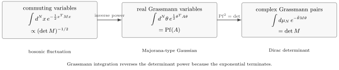
Ordinary commuting Gaussian integrals produce inverse determinant powers, while Grassmann Gaussian integrals produce determinant powers. This reversal is ultimately caused by $\theta^2=0$: the exponential terminates, so the integral selects the top coefficient rather than averaging over a continuum.

Pfaffians and the four-variable test

The Pfaffian is the natural answer for a Gaussian in real Grassmann variables. The first nontrivial case has two variables. For

$$A=\begin{pmatrix} 0&a\\ -a&0 \end{pmatrix},$$

we have

$$\frac12\theta_iA_{ij}\theta_j=a\theta_1\theta_2,$$

so

$$\int d\theta_2d\theta_1\,e^{a\theta_1\theta_2} =\int d\theta_2d\theta_1(1+a\theta_1\theta_2)=a.$$

Thus $\operatorname{Pf}(A)=a$.

For four variables, the Pfaffian is the signed sum over pairings:

$$\operatorname{Pf}(A)=A_{12}A_{34}-A_{13}A_{24}+A_{14}A_{23}.$$

That is exactly the same sign pattern as the fermionic Wick theorem for four fields. Grassmann Gaussians know about fermionic signs automatically.

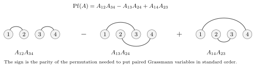
The four-variable Pfaffian is the signed pairing sum $A_{12}A_{34}-A_{13}A_{24}+A_{14}A_{23}$. The same alternating signs appear in fermionic Wick contractions.

Gaussian expectation values

Take an even finite number of real Grassmann generators and an invertible antisymmetric matrix $A$. Its Pfaffian is then nonzero, so the normalized expectation value is defined by

$$\langle \mathcal O(\theta)\rangle_A =\frac{\int d^N\theta\,\mathcal O(\theta) \exp\left(\frac12\theta_iA_{ij}\theta_j\right)} {\int d^N\theta\, \exp\left(\frac12\theta_iA_{ij}\theta_j\right)}.$$

With the measure convention above, the two-point function is

$$\langle\theta_i\theta_j\rangle_A=(A^{-1})_{ji}.$$

The reversed order on the indices is a convention-dependent bookkeeping detail; the invariant statement is that the contraction is the inverse of the quadratic form, with the sign fixed by the chosen ordering of variables and measure.

For four variables one obtains

$$\begin{aligned} \langle\theta_i\theta_j\theta_k\theta_l\rangle_A &=\langle\theta_i\theta_j\rangle_A\langle\theta_k\theta_l\rangle_A -\langle\theta_i\theta_k\rangle_A\langle\theta_j\theta_l\rangle_A \\ &\quad +\langle\theta_i\theta_l\rangle_A\langle\theta_j\theta_k\rangle_A. \end{aligned}$$

The middle term has a minus sign because pairing $i$ with $k$ requires moving an odd object through another odd object. Higher correlation functions are Pfaffians of the matrix of two-point contractions.

For finitely many complex Grassmann pairs, take $M$ invertible before normalizing the weight $e^{-\bar\theta M\theta}$. With the one-pair convention stated above, the basic contraction is

$$\langle\theta_i\bar\theta_j\rangle=(M^{-1})_{ij},$$

and Wick’s theorem says that a product with equal numbers of $\theta$ and $\bar\theta$ variables is the signed sum over all $\theta$–$\bar\theta$ pairings. In determinant form, an alternating displayed order gives

$$\langle\theta_{i_1}\bar\theta_{j_1}\cdots \theta_{i_n}\bar\theta_{j_n}\rangle =\det\left[(M^{-1})_{i_a j_b}\right]_{a,b=1}^n,$$

where the rows and columns inherit the written $i_a$ and $j_b$ orders. Grouping all unbarred variables before all barred variables requires $n(n-1)/2$ odd interchanges and therefore gives

$$\langle\theta_{i_1}\cdots\theta_{i_n} \bar\theta_{j_1}\cdots\bar\theta_{j_n}\rangle =(-1)^{n(n-1)/2} \det\left[(M^{-1})_{i_a j_b}\right].$$

This explicit factor is safer than saying “up to a sign”: the displayed order fixes the sign completely.

Sources and the fermionic generating functional

The quickest way to derive fermionic Wick’s theorem is to introduce Grassmann sources. Let $\eta_i$ and $\bar\eta_i$ be external Grassmann variables that anticommute with $\theta_i$ and $\bar\theta_i$, and retain an invertible finite $M$. The finite-dimensional Gaussian identity is

$$Z[\bar\eta,\eta] =\int d\mu_N\, \exp\left(-\bar\theta M\theta+\bar\eta\theta+\bar\theta\eta\right) =(\det M)\exp\left(\bar\eta M^{-1}\eta\right),$$

with the same measure convention as above. The proof is the same completion of the square used for bosons, except that one must preserve the order of Grassmann objects:

$$-\bar\theta M\theta+\bar\eta\theta+\bar\theta\eta =-(\bar\theta-\bar\eta M^{-1})M(\theta-M^{-1}\eta) +\bar\eta M^{-1}\eta.$$

The determinant and source completion are developed in Schwartz 2014, § 14.6, pp. 270–272, Eqs. (14.87)–(14.100). His grouped measure is not substituted for this page’s paired measure; the declared one-pair normalization fixes our signs. The canonical Grassmann treatment supplies the finite-kernel and zero-mode qualifications.

Functional derivatives with respect to sources then generate correlation functions. Since $Z$ is an exponential of a bilinear source term, every derivative pairing pulls down one inverse matrix $M^{-1}$, and the signs are precisely the signs of the required source permutations.

For real calculations, the safest convention is to choose an ordering of the external fields first and then differentiate sources in the corresponding reverse order. Memorized determinant formulas are useful, but they do not replace the sign bookkeeping imposed by the displayed order of the fields.

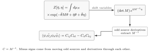
The free fermion generating functional is a determinant times an exponential quadratic in Grassmann sources. Source derivatives extract propagators. The signs are fixed by the order in which odd derivatives and odd sources are moved past one another.

The Dirac path integral

For the Dirac field, the variables $\psi_\alpha(x)$ and $\bar\psi_\alpha(x)$ in the path integral are independent Grassmann fields. The Lorentzian free action is

$$S_0[\bar\psi,\psi]=\int d^4x\,\bar\psi(x)(i\gamma^\mu\partial_\mu-m)\psi(x).$$

First choose a finite regulated kernel $K_{F,R}$ with the compatible vacuum boundary prescription and no unresolved zero modes. The finite quadratic action is $\bar\psi_I(K_{F,R})_{IJ}\psi_J$; the Gaussian identity applies with $M=-iK_{F,R}$ and sources $i\bar\eta,i\eta$. The spacetime expressions below denote the resulting kernels and their distributional limits when those limits exist. The source-dependent generating functional can be written schematically as

$$Z_0[\bar\eta,\eta] =\int\mathcal D\bar\psi\,\mathcal D\psi\, \exp\left\{iS_0[\bar\psi,\psi]+i\int d^4x\,[\bar\eta\psi+\bar\psi\eta]\right\}.$$

Let $K_F^{-1}$ denote the Feynman inverse of the Dirac operator $K=i\gamma^\mu\partial_\mu-m$. Thus

$$K_F^{-1}(p)=\frac{\gamma\cdot p+m}{p^2-m^2+i\epsilon}, \qquad S_F(p)=iK_F^{-1}(p).$$

The Gaussian shift then gives

$$\begin{aligned} \frac{Z_0[\bar\eta,\eta]}{Z_0[0,0]} &=\exp\left(-i\int d^4x\,d^4y\, \bar\eta(x)K_F^{-1}(x-y)\eta(y)\right) \\ &=\exp\left(-\int d^4x\,d^4y\, \bar\eta(x)S_F(x-y)\eta(y)\right). \end{aligned}$$

Here

$$S_F(x-y)=\int\frac{d^4p}{(2\pi)^4} \frac{i(\gamma\cdot p+m)}{p^2-m^2+i\epsilon}e^{-ip\cdot(x-y)}$$

is the same Feynman propagator obtained in the operator formalism.

Different authors place factors of $i$ in the definition of the propagator and in the source terms differently. With the convention used here,

$$(i\gamma^\mu\partial_\mu-m)S_F(x-y)=i\delta^{(4)}(x-y),$$

so $K_F^{-1}=S_F/i$. This is why the source exponential contains $-\bar\eta S_F\eta$, not $-i\bar\eta S_F\eta$. The convention-independent statement is that the quadratic Dirac operator is inverted with the Feynman boundary condition.

For example,

$$\langle0|T\{\psi_\alpha(x)\bar\psi_\beta(y)\}|0\rangle =S_{F,\alpha\beta}(x-y),$$

and

$$\begin{aligned} &\langle0|T\{\psi_{\alpha_1}(x_1)\psi_{\alpha_2}(x_2) \bar\psi_{\beta_1}(y_1)\bar\psi_{\beta_2}(y_2)\}|0\rangle \\ &\qquad =S_{F,\alpha_1\beta_2}(x_1-y_2)S_{F,\alpha_2\beta_1}(x_2-y_1) -S_{F,\alpha_1\beta_1}(x_1-y_1)S_{F,\alpha_2\beta_2}(x_2-y_2), \end{aligned}$$

for the displayed ordering of fields. The relative minus sign is not an extra Feynman rule. It is just the Grassmann algebra.

Closed fermion loops

The determinant in the free Gaussian is already hinting at a loop expansion. In Euclidean signature, if a fermion couples to a background bosonic field through an operator $D+V$, integrating out the fermion gives

$$\int\mathcal D\bar\psi\,\mathcal D\psi\, \exp\left(-\bar\psi(D+V)\psi\right) =\det(D+V).$$

Writing the determinant as an exponential,

$$\det(D+V)=\det D\, \exp\operatorname{Tr}\log(1+D^{-1}V),$$

and expanding the logarithm gives

$$\operatorname{Tr}\log(1+D^{-1}V) =\operatorname{Tr}(D^{-1}V) -\frac12\operatorname{Tr}(D^{-1}VD^{-1}V) +\frac13\operatorname{Tr}(D^{-1}VD^{-1}VD^{-1}V)-\cdots.$$

The trace is a loop: the propagators and vertices form a closed chain. To read off its statistics sign, include the determinant in the bosonic effective action:

$$e^{-S_{\mathrm{eff}}}=e^{-S_{\mathrm b}}\det(D+V), \qquad S_{\mathrm{eff}}=S_{\mathrm b}-\operatorname{Tr}\log(D+V).$$

The minus in front of $\operatorname{Tr}\log$ is the uniform extra minus associated with a closed fermion loop. The alternating coefficients in the expansion of $\log(1+D^{-1}V)$ are the separate algebraic coefficients of the logarithm and should not be mistaken for the statistics sign itself.

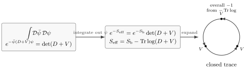
Integrating out a quadratic fermion gives $\det(D+V)$, hence $S_{\mathrm{eff}}=S_{\mathrm b}-\operatorname{Tr}\log(D+V)$. Expanding the trace-log produces closed chains of propagators and vertices; the overall minus is the fermion-loop statistics sign.

Summary

Grassmann variables are anticommuting algebraic variables. Their square is zero, so every function of finitely many Grassmann variables is a finite polynomial. Differentiation is graded, and Berezin integration is defined by coefficient extraction:

$$\int d\theta\,1=0, \qquad \int d\theta\,\theta=1.$$

This definition is not arbitrary decoration. It is the unique shift-invariant integral, up to normalization, and it is exactly what is needed to represent fermionic signs in a path integral.

The central Gaussian facts are

$$\int d^N\theta\,e^{\frac12\theta A\theta}=\operatorname{Pf}(A), \qquad \operatorname{Pf}(A)^2=\det A,$$

for real Grassmann variables, and

$$\int d\mu_N\,e^{-\bar\theta M\theta}=\det M$$

for complex Grassmann pairs. These formulas are the fermionic analogues of ordinary Gaussian integration, but the determinant powers are reversed relative to bosons.

Fermionic Wick’s theorem follows from the Grassmann Gaussian with sources. Correlation functions are signed sums over pairings, with signs determined by the number of odd interchanges required to bring paired variables together. In field theory, the Feynman propagator is $S_F=iK_F^{-1}$, with the vacuum boundary prescription on the inverse. Integrating out quadratic regulated fermions produces determinants whose logarithms generate closed fermion loops.

Common pitfalls

The most common mistake is to treat Grassmann variables as tiny ordinary numbers. They are not. They anticommute, and the sign obtained by moving one odd object through another is part of the calculation.

Another frequent mistake is to forget that the order of the measure matters. A formula such as

$$\int d\theta_2d\theta_1\,\theta_1\theta_2=1$$

is a convention. If one reverses the measure, the sign changes. Physical answers are unaffected only when all formulas are changed consistently.

It is also easy to confuse real and complex Grassmann Gaussians. Real Grassmann variables with an antisymmetric quadratic form give a Pfaffian. Complex Dirac-type pairs $\bar\theta,\theta$ give a determinant. Majorana fermions therefore naturally lead to Pfaffians, while Dirac fermions naturally lead to determinants.

Finally, $\bar\psi$ in the path integral is independent of $\psi$. It is not the complex conjugate of $\psi$ in the ordinary-number sense. The notation is chosen because it matches the Dirac adjoint in correlation functions and actions, but the integration variables are independent Grassmann generators.

Do not double-count the closed-loop sign. In diagrammatic perturbation theory a closed fermion loop carries a minus sign. In the path-integral derivation, that sign is already encoded by $S_{\mathrm{eff}}=S_{\mathrm b}-\operatorname{Tr}\log(D+V)$; it is not an extra sign to append after doing the Grassmann calculation.

Exercises

Exercise 1: translation invariance

Let $f(\theta)=a+b\theta$, with $a$ and $b$ Grassmann-even. Show that Berezin integration is translation invariant:

$$\int d\theta\,f(\theta+\rho)=\int d\theta\,f(\theta),$$

where $\rho$ is another Grassmann variable independent of $\theta$.

Solution

Because $f$ is linear,

$$f(\theta+\rho)=a+b\theta+b\rho.$$

Using

$$\int d\theta\,1=0, \qquad \int d\theta\,\theta=1,$$

and treating $b\rho$ as independent of $\theta$, we get

$$\int d\theta\,f(\theta+\rho) =a\int d\theta\,1+b\int d\theta\,\theta+b\rho\int d\theta\,1=b.$$

But

$$\int d\theta\,f(\theta)=a\int d\theta\,1+b\int d\theta\,\theta=b.$$

Thus the integral is translation invariant.

Exercise 2: the four-variable Pfaffian

Using the convention

$$\int d\theta_4d\theta_3d\theta_2d\theta_1\,\theta_1\theta_2\theta_3\theta_4=1,$$

show that

$$\int d^4\theta\,\exp\left(\frac12\theta_iA_{ij}\theta_j\right) =A_{12}A_{34}-A_{13}A_{24}+A_{14}A_{23},$$

where $A$ is antisymmetric.

Solution

Since $A_{ij}=-A_{ji}$,

$$\frac12\theta_iA_{ij}\theta_j =A_{12}\theta_1\theta_2+A_{13}\theta_1\theta_3+A_{14}\theta_1\theta_4 +A_{23}\theta_2\theta_3+A_{24}\theta_2\theta_4+A_{34}\theta_3\theta_4.$$

Only the quadratic term in the exponential can contain all four variables:

$$\exp(Q)=1+Q+\frac12Q^2, \qquad Q=\frac12\theta_iA_{ij}\theta_j.$$

The terms in $Q^2/2$ that contain $\theta_1\theta_2\theta_3\theta_4$ are the products of complementary pairings:

$$(A_{12}\theta_1\theta_2)(A_{34}\theta_3\theta_4),$$ $$(A_{13}\theta_1\theta_3)(A_{24}\theta_2\theta_4),$$

and

$$(A_{14}\theta_1\theta_4)(A_{23}\theta_2\theta_3),$$

including both orders from $Q^2$; the factor $1/2$ cancels this duplication. Reordering each monomial to $\theta_1\theta_2\theta_3\theta_4$ gives

$$\theta_1\theta_2\theta_3\theta_4, \qquad \theta_1\theta_3\theta_2\theta_4=-\theta_1\theta_2\theta_3\theta_4,$$

and

$$\theta_1\theta_4\theta_2\theta_3=+\theta_1\theta_2\theta_3\theta_4.$$

Therefore the coefficient of the top monomial is

$$A_{12}A_{34}-A_{13}A_{24}+A_{14}A_{23}.$$

The Berezin integral extracts exactly this coefficient.

Exercise 3: a two-pair determinant

For two complex Grassmann pairs, prove directly that

$$\int d\bar\theta_1d\theta_1d\bar\theta_2d\theta_2\, \exp(-\bar\theta_iM_{ij}\theta_j)=\det M,$$

using a measure convention normalized so that the one-pair formula gives

$$\int d\bar\theta\,d\theta\,e^{-\bar\theta\theta}=1.$$

Solution

The exponential terminates. Only the term containing all four variables contributes. Write

$$Q=-\bar\theta_iM_{ij}\theta_j.$$

Then

$$e^Q=1+Q+\frac12Q^2+\cdots,$$

and only $Q^2/2$ can contribute to the top monomial. Expanding the relevant terms gives two possibilities:

$$(\bar\theta_1M_{11}\theta_1)(\bar\theta_2M_{22}\theta_2)$$

and

$$(\bar\theta_1M_{12}\theta_2)(\bar\theta_2M_{21}\theta_1).$$

With the stated measure normalization, the first contributes $M_{11}M_{22}$ and the second contributes $-M_{12}M_{21}$. Hence

$$\int d\bar\theta_1d\theta_1d\bar\theta_2d\theta_2\,e^{-\bar\theta M\theta} =M_{11}M_{22}-M_{12}M_{21}=\det M.$$

Different orderings of the measure change intermediate signs, but the determinant formula is restored by using the corresponding one-pair normalization consistently.

Exercise 4: the Wick sign from sources

Let

$$Z[\bar\eta,\eta]=\det M\,\exp(\bar\eta_i(M^{-1})_{ij}\eta_j).$$

Use source derivatives to show that the normalized four-point function has the determinant sign pattern

$$\langle\theta_i\bar\theta_j\theta_k\bar\theta_l\rangle =(M^{-1})_{ij}(M^{-1})_{kl}-(M^{-1})_{il}(M^{-1})_{kj},$$

for the displayed order of variables.

Solution

The normalized generating functional is

$$\mathcal Z[\bar\eta,\eta]=\frac{Z[\bar\eta,\eta]}{Z[0,0]} =\exp(\bar\eta_aC_{ab}\eta_b), \qquad C=M^{-1}.$$

All derivatives are left derivatives, with the rightmost operator acting first. The two-point function is

$$\langle\theta_i\bar\theta_j\rangle =\left.\partial_{\eta_j}^L\partial_{\bar\eta_i}^L\mathcal Z\right|_0 =C_{ij}.$$

For the four-point function, expand the exponential to second order:

$$\mathcal Z=1+\bar\eta_aC_{ab}\eta_b+\frac12 (\bar\eta_aC_{ab}\eta_b)(\bar\eta_cC_{cd}\eta_d)+\cdots.$$

The four ordered derivatives corresponding to the insertion

$$\theta_i\bar\theta_j\theta_k\bar\theta_l$$

are $\partial_{\eta_l}^L\partial_{\bar\eta_k}^L\partial_{\eta_j}^L\partial_{\bar\eta_i}^L$. To see the signs before setting the sources to zero, the first two give

$$\partial_{\eta_j}^L\partial_{\bar\eta_i}^L\mathcal Z =C_{ij}\mathcal Z -\sum_{a,b}C_{ia}C_{bj}\bar\eta_b\eta_a\mathcal Z.$$

Applying $\partial_{\bar\eta_k}^L$ and then $\partial_{\eta_l}^L$ gives $C_{ij}C_{kl}$ from the first term and $-C_{il}C_{kj}$ from the second; terms still containing sources vanish at zero. Therefore

$$\langle\theta_i\bar\theta_j\theta_k\bar\theta_l\rangle =C_{ij}C_{kl}-C_{il}C_{kj}.$$

Substituting $C=M^{-1}$ gives the stated result.

Exercise 5: the trace-log and the closed-loop sign

Show that integrating out a fermion coupled to a background interaction $V$ gives a sum of closed-loop traces:

$$\log\frac{\det(D+V)}{\det D} =\sum_{n=1}^\infty\frac{(-1)^{n+1}}{n}\operatorname{Tr}(D^{-1}V)^n.$$

Then explain why these terms enter the Euclidean bosonic effective action with an overall minus sign.

Solution

First factor out $D$:

$$\frac{\det(D+V)}{\det D}=\det(1+D^{-1}V).$$

Taking the logarithm gives

$$\log\frac{\det(D+V)}{\det D} =\operatorname{Tr}\log(1+D^{-1}V).$$

Now use the ordinary matrix identity

$$\log(1+X)=X-\frac12X^2+\frac13X^3-\cdots,$$

with $X=D^{-1}V$. Hence

$$\operatorname{Tr}\log(1+D^{-1}V) =\sum_{n=1}^\infty\frac{(-1)^{n+1}}{n}\operatorname{Tr}(D^{-1}V)^n.$$

Each trace is cyclic and therefore corresponds diagrammatically to a closed chain of propagators $D^{-1}$ and insertions $V$.

Finally,

$$e^{-S_{\mathrm{eff}}}=e^{-S_{\mathrm b}}\det(D+V)$$

implies

$$S_{\mathrm{eff}}=S_{\mathrm b}-\operatorname{Tr}\log(D+V).$$

Therefore the entire trace-log contribution carries the extra minus associated with a closed fermion loop. This statistics sign is distinct from the alternating powers generated by expanding $\log(1+X)$.

References

• Schwartz, Matthew D. Quantum Field Theory and the Standard Model. Cambridge University Press, 2014. DOI.

Further reading

• Berezin, Felix A. The Method of Second Quantization. Academic Press, 1966, chapter 1.
• Coleman, Sidney. Lectures of Sidney Coleman on Quantum Field Theory. Edited by Bryan Gin-ge Chen et al. World Scientific, 2019, chapter 29.
• Di Francesco, Philippe, Pierre Mathieu, and David Sénéchal. Conformal Field Theory. Springer, 1997, appendix 2.B.
• Srednicki, Mark. Quantum Field Theory. Cambridge University Press, 2007, sections 43–44.
• Zee, Anthony. Quantum Field Theory in a Nutshell. 2nd ed., Princeton University Press, 2010, chapter II.5 and appendix A.